Node properties sheets allow for modifying properties of model nodes. They can be opened in the following two ways:
1. Double-click on a node in the Graph View.
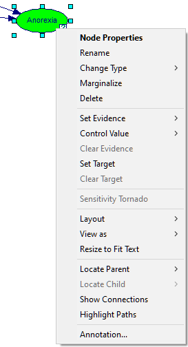
2. Right click on the name of the node in the Tree View or right click on the icon of the node in the Graph View. This will display the Node Pop-up menu. Select Node Properties from the menu.
The Node properties consist of several tabs. While we will discuss all of the tabs in this section, not all of the tabs appear among the Node properties at the same time. The Value tab appears only when the value of the node is available. Some tabs appear only when the diagnostic features of GeNIe are enables.
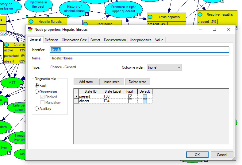
General tab
General tab is the first tab of the Node properties. Shown below is a snapshot of the General tab when the diagnostic options are disabled:
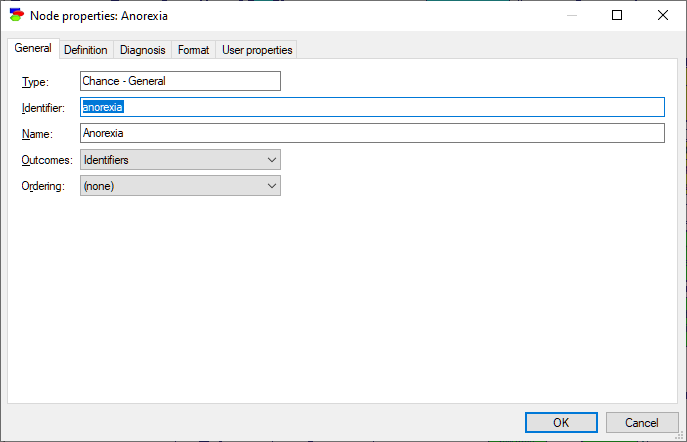
The General tab contains the following properties:
Node Type (in the picture, it is Chance - General) cannot be changed in the General tab and serves only informational purpose. Node type is selected during node creation (by selecting the appropriate icon from the Standard Toolbar). It can be changed after creation by either right clicking on the node in the Graph View and selecting Change Type... from the Node Pop-up menu or selecting Change Type from the Node Menu in the Menu Bar. This will display a sub-menu from which you can choose the new type for the node. See Node Menu section for more information.
Identifier displays the identifier for the node, which is user-specified. Identifiers must start with a letter, and can contain letters, digits, and underscore (_) characters. Letters are a-z and A-Z but also all Unicode characters above codepoint 127, which allows using characters from other alphabets than the Latin alphabet. The identifier for the network shown above is anorexia.
Name displays the name for the network, which is user-specified. There are no limitations on the characters that can be part of the name. The name for the network shown above is Anorexia.
The reason for having both, the Identifier and the Name is that nodes may be referred to in equations. In that case, the reference should avoid problems with parsing, which could easily appear with spaces or special characters. On the other hand, Identifiers, which are meant to refer to nodes, may be too cryptic when working with a model, so we advise that Names be used for purposes such as displaying nodes.
Outcomes allows for specifying the type of outcomes that the node will have. There are four basic types of outcomes
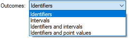
Identifiers are those nodes that consist of categorical states, Intervals and Point values (possibly with Identifiers) allow for specifying discrete numerical nodes. We will discuss each of these sub-types in the Definition tab section below.
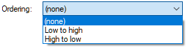
Ordering gives the modeler the opportunity to indicate whether the outcomes of the node are sorted from the highest to the lower or lowest to the highest value. This becomes important in some types of nodes, for example in canonical models.
Definition tab
Definition tab allows for specifying node definition, i.e., how the node interacts with other nodes in the model. While there are common elements among various definition tabs, there are as many definition tabs as there are combinations of node kinds, domains, and probability types.
Chance nodes: Identifiers
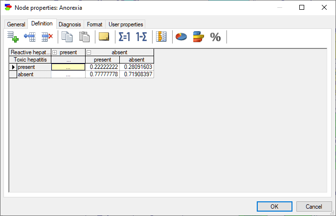
Chance nodes specified as Identifiers allow for modeling discrete random variables that have categorical outcomes described by labels. Their definition consists of a set of conditional probability distributions, one for each combination of the parents' outcomes, and collected in a table names conditional probability table (CPT). (In case of Noisy-MAX nodes, the definition is slightly different but it is equivalent to a CPT.)
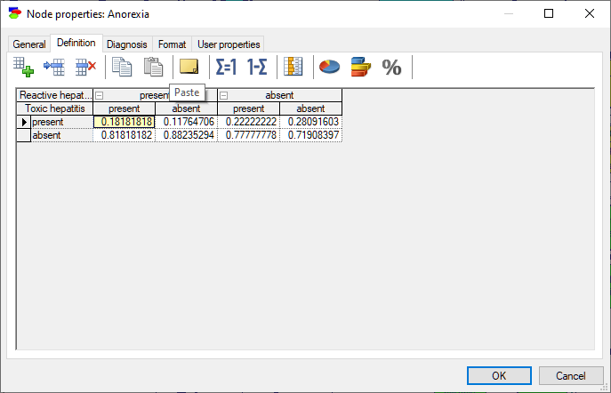
The rows of the table correspond to states of the random variable modeled by the node (in this case, Anorexia). The state names can be changed by clicking on them. The top rows, with gray background correspond each to a parent of Anorexia: Reactive hepatitis and Toxic hepatitis. Because each of the variables involved in this interaction is binary and there are two parents, we have 2x2=4 columns in the CPT. Each column corresponds to one combination of outcomes of the parents. For example, the first column from the left corresponds to Reactive hepatitis being present and Toxic hepatitis being present. The order of parents can be changed by dragging and dropping them in their new position, which may prove useful in probability elicitation, as some orders may turn out to be counter-intuitive. The order of states in the table can be changed by dragging and dropping as well. Individual probabilities can be edited by clicking on them. There are several convenient tools that help with filling the tables with probabilities:
Add (![]() ), Insert (
), Insert (![]() ), and Delete (
), and Delete (![]() ) buttons are useful in adding and removing states. They add a new state after the selected state, add a new state before the selected state, and delete the selected state, respectively.
) buttons are useful in adding and removing states. They add a new state after the selected state, add a new state before the selected state, and delete the selected state, respectively.
Copy (![]() ) and Paste (
) and Paste (![]() ) buttons allow for copying and pasting fragments of the definition spreadsheet. Please note that GeNIe allows for copying and pasting to and from other programs on your computer, for example Microsoft Excel.
) buttons allow for copying and pasting fragments of the definition spreadsheet. Please note that GeNIe allows for copying and pasting to and from other programs on your computer, for example Microsoft Excel.
Tip: You can select the entire spreadsheet quickly by clicking on the Node name, or an entire column by clicking on the state name. You can also select the spreadsheet by having the cursor in any of the cells and pressing CTRL-A. You can select all state names quickly by having the cursor in any of the names and pressing CTRL-A.
The Quickbar (![]() ) button turns on graphical display of the probabilities in the background. It is useful for visualizing the order of magnitude of numerical probabilities.
) button turns on graphical display of the probabilities in the background. It is useful for visualizing the order of magnitude of numerical probabilities.
The Annotation (![]() ) button (shortcut CTRL+T) allows for adding annotations to state names and to individual probabilities. Please use it generously, as models are best viewed as documents of your decision problem.
) button (shortcut CTRL+T) allows for adding annotations to state names and to individual probabilities. Please use it generously, as models are best viewed as documents of your decision problem.
The Normalize (![]() ) and Complement (
) and Complement (![]() ) buttons are useful when entering probability distributions.
) buttons are useful when entering probability distributions.
The Normalize button (shortcut CTRL+N) normalizes the contents of the selected column by dividing each number by the sum of all numbers in the column. The effect of this operation is that the sum of all numbers in the column becomes precisely 1.0, something that is expected of a probability distribution. This button makes it convenient to enter probabilities as percentages (e.g., 10, 30, and 70), then selecting the column and pressing the Normalize button, which changes the numbers to (0.1, 0.3, and 0.7) so that they are a correct probability distribution.
The Complement button (shortcut CTRL+O) can be pressed after selecting one or more cells (they do not have to be cells in the same column). When pressed, it fills in the selected cell the complement of the remaining cells in the column, i.e., a number that will make the sum equal precisely to 1.0. For example, in the simplest case, when two of the three cells contain 0.1 and 0.3 and the Complement button is pressed with the third cell selected, the cell will receive 0.6, which is 1.0-(0.1+0.3). When multiple cells within a column are selected, GeNIe will distribute the complement among the selected cells using the existing values as weights when distributing. Here is an example: Let the probabilities in a column be (0.4, 0.3, 0.4, 0.2). If the last two cells (with 0.4 and 0.2) are selected when the Complement button is pressed, the probabilities will change to (0.4, 0.3, 0.2, 0.1). The complement probability (1-0.4-0.3=0.3) gets distributed between the selected cells in the proportion 0.4:0.2 or 2:1, yielding 0.2 and 0.1. When cells in multiple columns are selected, the complement operation will be performed in each of the columns with selected cells in separation. Pressing the Complement button will lead to an error message if the sum of probabilities of the other fields in the column exceeds 1.0. The buttons saves typing and ensures that the probability distribution is correct.
It is possible to use the cell-oriented probability distribution interface as a simple calculator by typing in a cell a mathematical expressions preceded by the = character. Such expressions are evaluated immediately and the result of the evaluation is placed in the cell. For example, typing in the cell =1/3 will evaluate to a floating point number 0.33333333. It also works with functions and probability distributions (see the Writing equations in GeNIe section for a list of functions and distributions known by GeNIe). For example, typing =Uniform(0,1) will result in a single random number from the Uniform(0,1) distribution, e.g., 0.39330341.
GeNIe warns the user of problems in the probability distribution tables whenever these contain incorrect distributions. Any number outside of the range [0..1] causes GeNIe to raise a flag in the cell. Also, when the sum of probabilities in a column is not 1.0, GeNIe places a flag on the column.
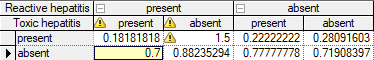
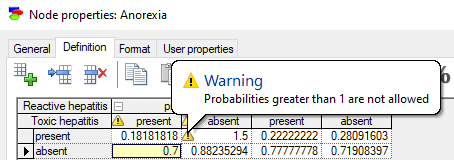
Hovering the mouse over the flag displays a warning message with the reason for the flag. Probabilities greater than 1.0 result in the following warning:
Sum of probabilities not equal to 1.0 results in the following warning:
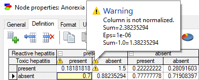
The warning displays the sum of probabilities, the tolerance threshold value (in the above example Eps=1e-06=0.000001), and the difference between the sum and the theoretically enforced sum of 1.0. The tolerance threshold is adaptive and is never larger than the smallest probability value in the CPT.
GeNIe will not allow to exit the Node properties dialog if the definition is incorrect.
Finally, it is possible to enter probability distributions graphically, either through a probability wheel or a bar chart. Pressing on the Elicitation piechart (![]() ) button invokes a probability wheel dialog:
) button invokes a probability wheel dialog:
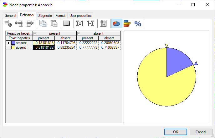
You can modify the probability distribution graphically using the small triangles. Drag a triangle around the circumference of the pie to increase or decrease the probability distribution for that state. As we adjust the size of one section of the piechart, the remaining section change proportionally. In case of variables with multiple states, it is sometimes useful to lock a selected part of the piechart to prevent it from changing. We can lock a part of the pie chart by right-clicking on the part and selecting Lock (or simply double-clicking on that part).
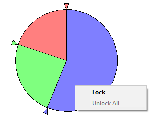
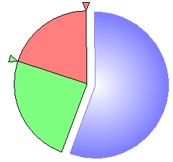
The effect of this is that the locked part shows as separate from the rest of the pie and no longer takes part in elicitation, remaining constant until released.
It is possible to lock multiple parts.
Elicitation barchart (![]() ) button invokes a similar graphical elicitation dialog but based on a bar chart:
) button invokes a similar graphical elicitation dialog but based on a bar chart:
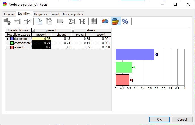
Here also you can change the size of the individual bars by dragging the small triangles on their right-hand side. You can lock those bars that we are happy with to prevent then from further changing.
The Show percentages in the elicitation chart (![]() ) button turns on a tool tip that shows the numerical value of the modified probability. There has been empirical research showing that viewing the probabilities during graphical elicitation may not be the best idea in terms of leading to a decreased accuracy of the elicitation.
) button turns on a tool tip that shows the numerical value of the modified probability. There has been empirical research showing that viewing the probabilities during graphical elicitation may not be the best idea in terms of leading to a decreased accuracy of the elicitation.
In case of both, the piechart and barchart, it is possible to elicit multiple columns at the same time. Just select the columns that you desire before entering the elicitation dialog. The resulting probability distributions will be entered in all the selected columns. The elicitation piechart and barchart are equivalent formally but are convenient for different purposes at the user interface. The barchart is better at showing the absolute value of probability while the piechart may be better at relative comparisons.
Sometimes, the order of parents or the order of states in a node may be not intuitive. GeNIe allows for an interactive change of the order of parents and states. Simply click on the parent name or the state name and drag it to its destination position.
When a CPT is very large, it is useful to shrink parts of it. To that effect, please use the small buttons in the header lines (![]() and
and ![]() ).
).
Chance nodes: Intervals
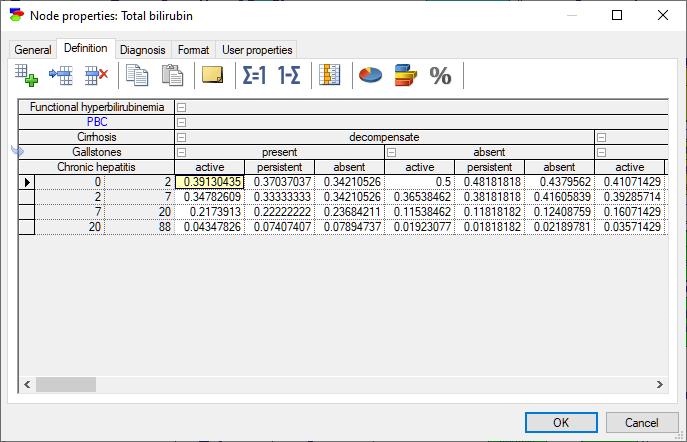
Chance nodes specified as Intervals or Identifiers with intervals allow for modeling discrete random variables that are numerical in nature. The domain of such variables is divided into adjacent intervals, with the borders specified explicitly, as in the variable below (the Definition tab is for a Chance-General node; definition tabs for other discrete chance nodes are similar):
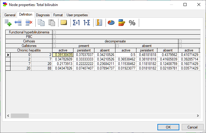
Nodes specified as Identifiers with intervals allow for naming each interval, in addition to specifying their boundaries.
The probability distribution over such variables is discrete and each interval is treated as a discrete state. For the purpose of numerical calculations, such as the calculation of the mean or standard deviation, the possible (numerical) values of the variable are assumed to be distributed uniformly within each of the intervals, except for open intervals, i.e., intervals with left boundary of -inf or right boundary of inf (empty cells act as -inf and inf, respectively). The definition of a variable that is specified as Intervals or Identifiers with intervals consists also of a set of conditional probability distributions, one for each combination of the parents' outcomes, and collected in a table names conditional probability table (CPT). All operations of the CPT are the same as in case of variables with Identifiers.
Chance nodes: Point values
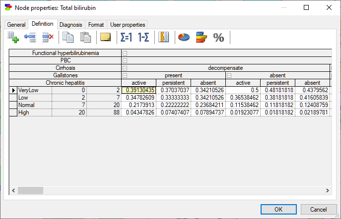
Chance nodes specified as Identifiers and point values allow for modeling discrete random variables that are numerical in nature. The domain of such variables is a set of discrete numerical values, as in the variable below:
Nodes specified as Identifiers and point values allow for naming each numerical point value, in addition to specifying the value itself.
The probability distribution over such variables is discrete and each (labeled) numerical value is treated as a discrete state. For the purpose of numerical calculations, such as the calculation of the mean or standard deviation, the possible (numerical) values of the variable are assumed to be distributed uniformly within each of the intervals, except for open intervals, i.e., intervals with left boundary of -inf or right boundary of inf (empty cells act as -inf and inf, respectively). The definition of a variable that is specified as Intervals or Identifiers with intervals consists also of a set of conditional probability distributions, one for each combination of the parents' outcomes, and collected in a table names conditional probability table (CPT). All operations of the CPT are the same as in case of variables with Identifiers.
Chance-NoisyMax nodes
Chance-NoisyMax are a special case of chance nodes modeling discrete random variables using the Noisy-Max assumption (please see the section Noisy-MAX model). Chance-Noisy-MAX nodes, similarly to Chance-General nodes, can have domains specified by Identifiers, Intervals, Identifiers and intervals, and Identifiers and point values. Their definition consists of a set of conditional probability distributions, one for each state of each parents' outcomes. The NoisyMax nodes allow for specification of the interaction with their parents in a simplified way, requiring fewer parameters. The specifications can be viewed as a conditional probability table (CPT).
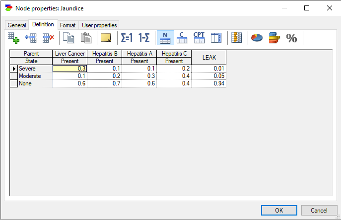
Most of this dialog resembles the dialog for the Chance-General nodes. The additional functionality, which we discuss below, allows for Noisy-MAX-specific activities. The buttons Show net parameters (![]() ) and Show compound parameters (
) and Show compound parameters (![]() ) switch between two representations of the Noisy-MAX parameters: net and loaded. Only one of the two buttons can be pressed at any given time. The Show CPT (
) switch between two representations of the Noisy-MAX parameters: net and loaded. Only one of the two buttons can be pressed at any given time. The Show CPT (![]() ) button shows the CPT that corresponds to the Noisy-MAX specification. Finally, the Show constrained columns (
) button shows the CPT that corresponds to the Noisy-MAX specification. Finally, the Show constrained columns (![]() ) button brings forward trivially-filled columns of the Noisy-MAX specification that are normally not needed to parametrize a Noisy-MAX distribution but are handy in case one wants to change the order of states of any of the parent variables. The order of states of the parent variables is changed here only in the context of the current definition definition of interaction between the node and its parents and does not impact the definitions of the parent variables. Please see the Noisy-MAX model section for a tutorial-like introduction to the Noisy-MAX gate.
) button brings forward trivially-filled columns of the Noisy-MAX specification that are normally not needed to parametrize a Noisy-MAX distribution but are handy in case one wants to change the order of states of any of the parent variables. The order of states of the parent variables is changed here only in the context of the current definition definition of interaction between the node and its parents and does not impact the definitions of the parent variables. Please see the Noisy-MAX model section for a tutorial-like introduction to the Noisy-MAX gate.
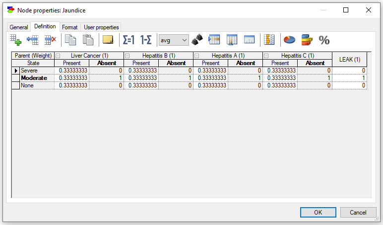
Chance-NoisyAdder nodes
The Noisy-Adder nodes are a special case of chance nodes modeling discrete random variables using the noisy-adder assumption. Chance-NoisyAdder nodes, similarly to Chance-General nodes, can have domains specified by Identifiers, Intervals, Identifiers and intervals, and Identifiers and point values. Noisy-Adder is a non-decomposable model that derives the probability of the effect by taking the average of probabilities of the effect given each of the causes in separation. Similarly to the Noisy-MAX nodes, noisy-adder nodes allow for specification of the interaction with their parents in a simplified way, requiring fewer parameters. The specifications can be viewed as a conditional probability table (CPT). Please see the Noisy-Adder model section for a tutorial-like introduction to the Noisy-Adder nodes.
Deterministic nodes
Deterministic nodes are discrete nodes that have no noise in them, i.e., we know their state with certainty if we know the states of their parents. Deterministic nodes, similarly to Chance-General nodes, can have domains specified by Identifiers, Intervals, Identifiers and intervals, and Identifiers and point values. The definition of a deterministic node is a truth table - knowing the values of the parents of a deterministic node defines its state. The only difference between a Chance-general node and a Deterministic node is that the values in the table of the latter are radio buttons rather than zeros and ones. Consider the following deterministic node expressing the relationship between class of an animal and its body covering. Once we know the class of the animal, we know the body covering: birds have down, mammals have hair, and reptiles have scales.
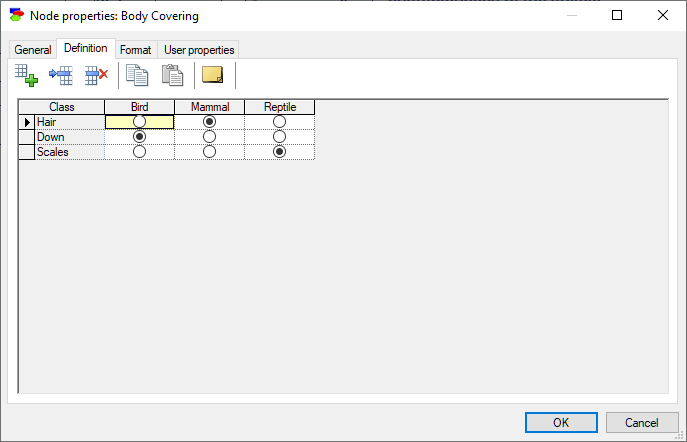
The definition corresponds to one in which we have 1.0 in exactly one of the cells of each column (the one with the radio button turned on) and zeros in all the other cells. All editing actions are the same as in Chance-general nodes.
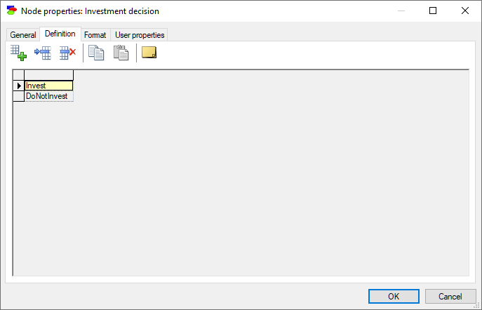
Decision nodes
Decision nodes are discrete nodes that are under control of the decision maker and, hence, have no parents influencing them and no numerical specification. Decision nodes, similarly to Chance-General nodes, can have domains specified by Identifiers, Intervals, Identifiers and intervals, and Identifiers and point values.
All editing actions are the same as in Chance-general nodes.
Utility nodes
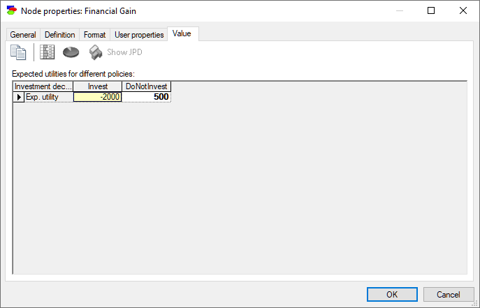
Utility nodes model decision maker's preferences for various states of their parents. Utility nodes are continuous and can assume any real values. When their parents are discrete, each cell in the value node defines a measure of preference of the combination of states of these parent nodes.
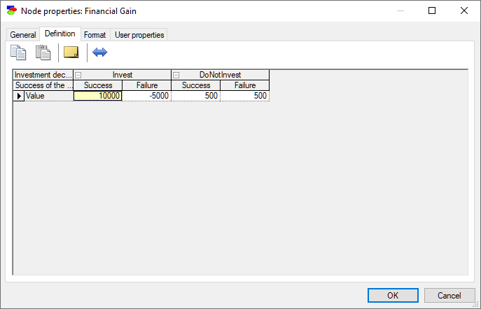
In the example above, node Financial Gain expresses the monetary gain for all combinations of states of the nodes Investment decision and Success of the venture. In expected utility theory, decisions are optimal when they maximize the expected utility. It turns out that the maximization process is independent on the unit and the scale of the utilities but only on their relative values. Utility values are determined up to a linear transformation. You can transform your utility function to a different scale by pressing the Linear transformation (![]() ) button, which will invoke the following dialog:
) button, which will invoke the following dialog:
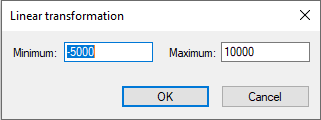
The fields Minimum and Maximum contain the lowest and the highest value in the table, respectively. When these values are edited and the OK button is pressed, the values in the table are linearly transformed to the new interval. This operation is useful in case the numbers in the table are utilities. Very often a decision modeler wants to have the utility function located in a given interval, usually [0..1] or [0..100].
ALU nodes
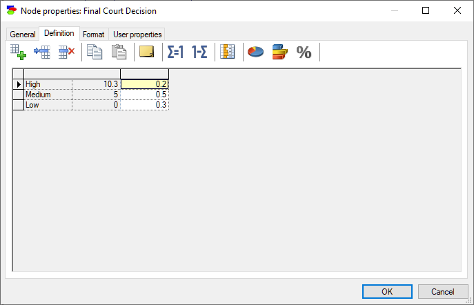
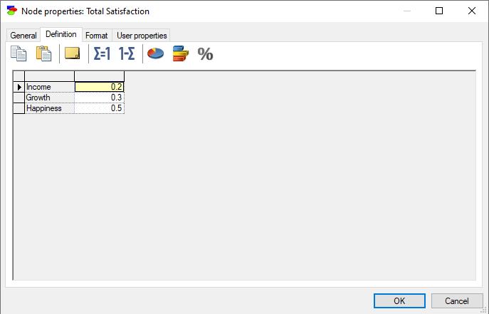
ALU or Additive-Linear Utility nodes are continuous nodes that model decomposable utility functions. An ALU node brings together utilities of several Utility nodes in an additively-linear function. Consider the following model, in which the node Total Satisfaction is a function of three utility nodes: Income, Growth and Happiness.
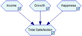
Let us assume that these combine linearly with weights 0.2, 0.3, and 0.5, respectively, i.e., we are dealing with the following function of the utilities of the three components: Total Satisfaction = 0.2 Income + 0.3 Growth + 0.5 Happiness. The following definition of an ALU node captures this interaction
All editing actions are the same as in Chance-general nodes. In particular, the Normalize (![]() ) and Complement (
) and Complement (![]() ) buttons are useful because it is customary to make the weights in an ALU function add up to 1.0. Because of this, GeNIe offers also graphical utility elicitation.
) buttons are useful because it is customary to make the weights in an ALU function add up to 1.0. Because of this, GeNIe offers also graphical utility elicitation.
MAU nodes
MAU or Multi-Attribute Utility nodes generalize the ALU nodes to any function of the parent utilities. The Definition tab of a MAU node looks as follows:
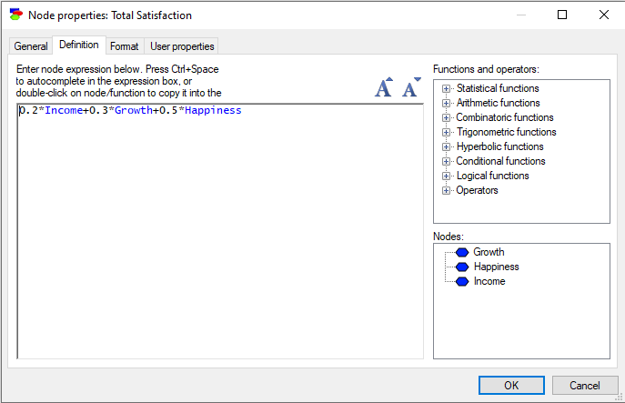
The dialog allows for entering any function of the parent utilities. The current definition shows the additive linear function corresponding to the example used for the ALU nodes. In addition to arithmetic operators, GeNIe offers a number of arithmetic, combinatoric, trigonometric, hyperbolic, and logical/conditional functions, which can be typed directly or selected from the lists in the right-hand side window pane. When editing an equation, press Ctrl+Space to auto complete in the Expression box or double-click on node/function to copy it into the equation. Pressing on the increase/decrease font size icons or using Ctrl+wheel allows to change the font size.
Equation nodes
Equation nodes are continuous chance nodes, whose interaction with their parents can be described by means of an equation. Equation nodes are a bridge between Bayesian networks and systems of simultaneous structural equations, popular in physics and engineering applications. The following dialog shows a variable describing the cold water outlet temperature of a building. It is described by the following equation:
Tcwout=mflowma*sp_heatair*(-Tsa+Tma)/(mdotcw*sp_heatwater)+Tcwin
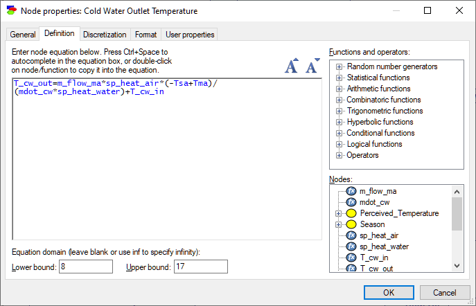
The window panes on the right-hand side of the tab contain a set of standard functions known by GeNIe and the set of nodes that participate in the equation. When editing an equation, press Ctrl+Space to auto complete in the Expression box or double-click on node/function to copy it into the equation. Pressing on the increase/decrease font size icons or using Ctrl+wheel allows to change the font size.
Another element of the dialog describes the domain of the variable, which is any real number between Lower bound and Upper bound. Because a complete freedom in the model specification prevents GeNIe from using an exact algorithm that will solve the model, the default algorithms are based on stochastic sampling. Specification of the domain of the variable helps in limiting the sampling domain and improves the algorithm efficiency, allowing for warnings in case values fall outside of the specified bounds. One or both domain bounds can be infinite. Just leave the corresponding box empty or enter the text -inf and inf, respectively.
While we will describe equation nodes in DBNs in section Creating a hybrid DBN, this is a good moment to introduce continuous/equations nodes as they are defined in DBNs. Continuous/equation nodes that are placed inside the temporal plate represent in general difference equations. GeNIe uses the following notation for references to different time steps. A variable name with curly brackets should have a time index inside the brackets. Time index is a formal variable with a possible offset. For example, in the definition of the variable R below,
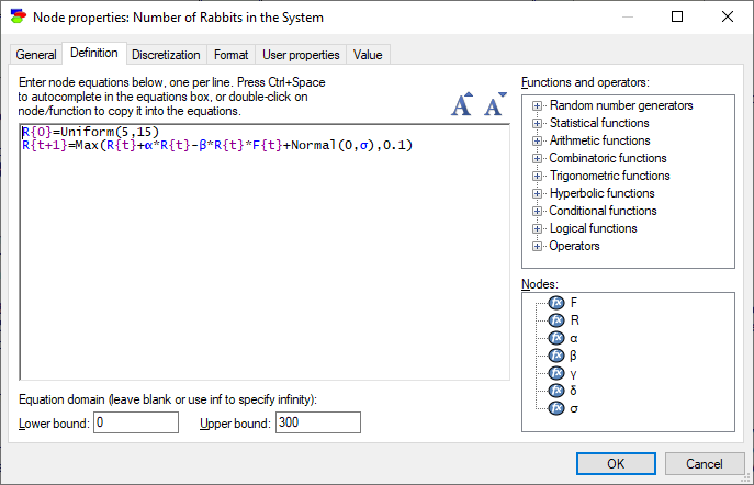
we have an equation:
R{t+1}=Max(R{t}+α*R{t}-β*R{t}*F{t}+Normal(0,σ),0.1)
The equation introduces a formal time variable t (this could be any label that is unique within the definition of R). R{t+1} refers to the value of that variable at time t+1 and the equation specifies that value in terms of the values of R{t} (R at time t) and F{t} (F at time t).
Because the equation involves a definition of the variable R at time t+1 in terms of its value at time t, we need an initial condition, i.e., the value of R at time 0. This is specified by the first equation
R{0}=Uniform(5,15)
As a general rule, there should be as many equations specifying initial conditions as the order of the difference equation. If the equation makes reference to {t+2}, two equations with initial conditions are needed.
Everything else in DBN continuous/equation nodes is the same as in static Bayesian networks, i.e., the equations may take any form and may use any function or probability distribution known by GeNIe, defined in the right-hand side of the tab.
Format tab
The Format tab is used to specify how the node will be displayed in the Graph View. It has a preview window which displays the altered view of the node with the new settings.
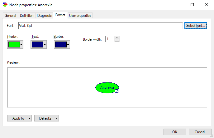
Select font button is used to select the font of the text displayed within the node. Clicking on this button will cause a standard Font Selection dialog box to be displayed. You can select font type, style, and size from this box.
Interior, Text, and Border colors allow for choosing the colors of the interior, font, and border colors, respectively. Clicking on any of these buttons brings up a color selection palette, example of which is shown below
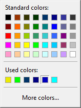
You can select any of the 40 palette colors or can bring up the possibility to select from more colors by clicking on More colors.... This will display a selection dialog as follows:
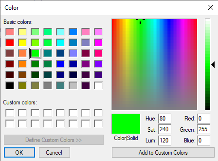
You can select any color on the rainbow-like part of the window and then add the selected color to one of the 16 custom colors (by clicking on the button Add to Custom Colors).
Border width allows to change the width (in pixels) of the border around the node. This parameter can be used to change the node visibility in the Graph View. The default width for most nodes is one pixel. Submodel nodes have borders of width two.
The Node properties dialog is powerful but unless you want the changes to apply only to one node that you have used to invoke the dialog, you need to make careful choices in two separate menus: the Apply to menu and the Defaults menu.
The Apply to menu gives two choices: Selected nodes and All nodes.
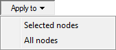
If you make no choice here, your changes will apply only to the current node (its name is displayed in the preview window). If you want to apply the changes to a group of nodes (selected before invoking this dialog), choose Selected nodes. If you want to apply the changes to all nodes in the network, choose All nodes. Generally, to change the formatting properties of a group of nodes, it is best to select them first (please consider using the corresponding selection commands from the Edit Menu or from the Diagnosis menu (nodes can be selected by type, diagnostic type, or color), once the diagnostic extensions are enabled) and then right-click on any of the selected nodes to invoke Node properties. (Invoking node properties by double-clicking on a node has a side-effect of selecting the node and clearing any existing selections.)
The Defaults pop-up menu allows you to modify the program defaults, which will make all new nodes appear the way you have specified. The menu gives you three choices: Set as Defaults, Set as Defaults (This Session Only), and Restore Defaults.
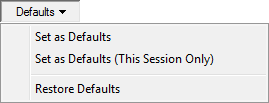
Set as Defaults set the new format as the default format for all new nodes. This default setting will be maintained between multiple sessions of GeNIe. Set as Defaults (This Session Only) makes the new setting a default but only for this session only. After you quit and start GeNIe again, the previous default settings will be restored. Restore Defaults restores the factory settings.
User properties tab
The User Properties tab allows the user to define properties of the node that can be later retrieved by an application program using SMILE. For example, the following tab for the node Anorexia contains two properties: Author with the value Agnieszka Onisko and Location with the value C:\Program Files\GeNIe 2.1\HeparII.xdsl. Neither GeNIe nor SMILE use these properties and they provide only placeholders for them. They are under full control and responsibility of the user and/or the application program using the model. GeNIe only allows for editing them.
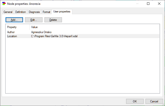
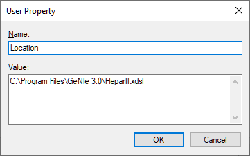
Both Add and Edit invoke the following dialog:
Delete removes the selected property.
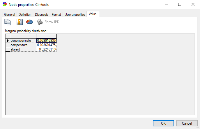
Value tab
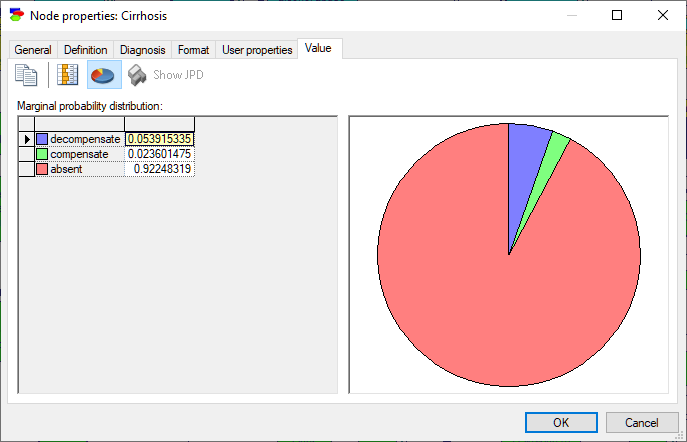
The Value tab is visible only if an algorithm has been applied to the model and the node contains the calculated values (typically, the marginal probability distribution or the expected utilities). The precise format for the Value tab depends on the node type.
Discrete Chance and Deterministic nodes show their marginal probability distributions.
To make the display graphical, press the Piechart (![]() ) and/or the Show QuickBars (
) and/or the Show QuickBars (![]() ) buttons. They add a pie chart display of the posterior marginal distribution and bars in the result spreadsheet (a list of states with their posterior probabilities) respectively.
) buttons. They add a pie chart display of the posterior marginal distribution and bars in the result spreadsheet (a list of states with their posterior probabilities) respectively.
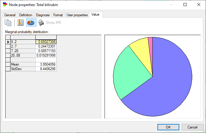
Nodes that are numerical but discrete show, in addition to probability distribution over its states, their mean and standard deviation.
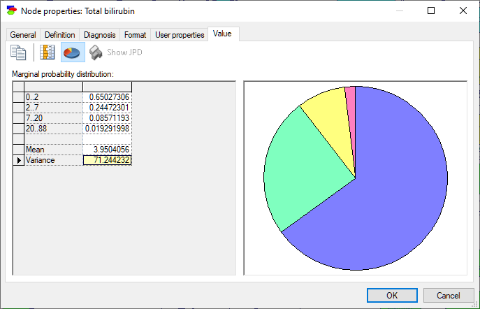
Standard deviation can be turned into variance by double-clicking on the row showing standard deviation:
Calculation of the mean and standard deviation/variance is straightforward in nodes with numerical point values. In case of interval nodes, GeNIe assumes that the distribution is uniform within each of the intervals.
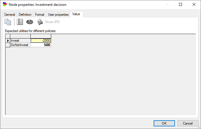
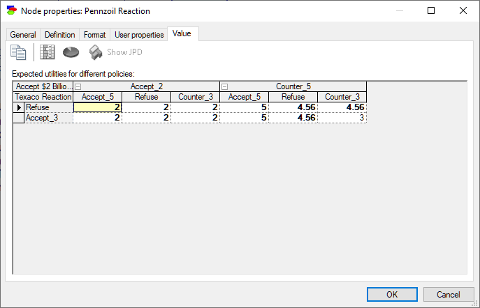
Decision, Utility, ALU and MAU nodes show expected utilities of each of the decision options. There is a subtle difference between the two displays in that Decision nodes show the result for each of the states of the decision node (rows of the result table) and in case of Utility nodes, states of the Decision node are indexing the result. Here is the value tab of a Decision node:
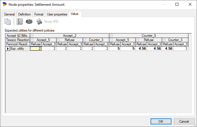
The same information shown by the Utility node of the same model:
When there are unobserved decision nodes that precede the current node or when there are unobserved chance nodes that should have been observed, GeNIe shows the results as a table indexed by the unobserved nodes.
The same information shown in the Utility node of the same model:
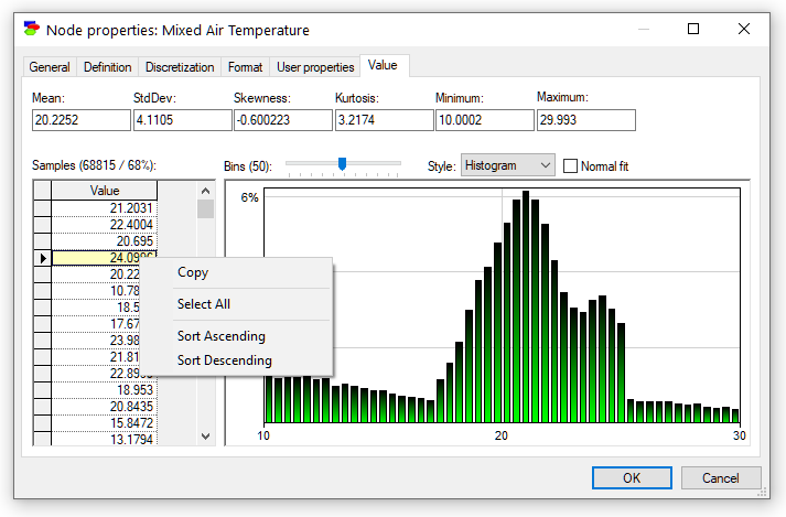
Equation nodes are continuous and show the results in form of a plot of the samples obtained during the most recent run of the sampling algorithm. The tab shows the first four moments of the distribution: Mean, StdDev, Skewness and Kurtosis along with the Minimum and the Maximum. By default, the plot shows the histogram of the samples:
Standard deviation can be turned into variance by double-clicking on the cell showing standard deviation
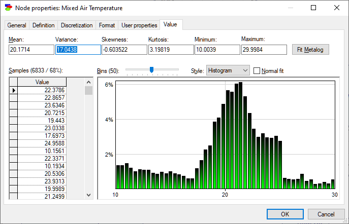
The samples themselves are preserved and displayed in the vector on the left-hand side. They can be selected, copied, and sorted using a right-click context pop-up menu (shown in the screen short). Similarly to the histogram interface in the data pre-processing module, the user can change the number of bins in the histogram.
Various toolbar buttons on the top of the tab allow for viewing the results in different ways. Show probability density function (![]() ) button shows the histogram of samples (this is the default), Show cumulative probability function (
) button shows the histogram of samples (this is the default), Show cumulative probability function (![]() ) button shows the cumulative histogram of samples, Display density function as line chart (
) button shows the cumulative histogram of samples, Display density function as line chart (![]() ) button changes both histograms into lines, Show normal distribution over density function (
) button changes both histograms into lines, Show normal distribution over density function (![]() ) button fits Normal distribution to the sample, and Fit metalog distribution (
) button fits Normal distribution to the sample, and Fit metalog distribution (![]() ) button invokes the Metalog Distribution dialog that allows for fitting a metalog distribution the samples.
) button invokes the Metalog Distribution dialog that allows for fitting a metalog distribution the samples.
With the AutoDiscretize algorithm used for inference in continuous models, the Value tab of Equation nodes is identical to those of Chance nodes.
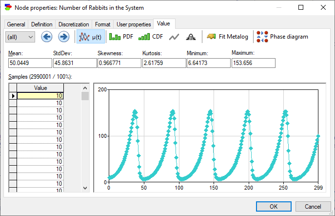
Equation nodes in DBNs look similar, although they show the result as a function of time. The default view shows the mean of the variable, although it is possible to view the PDF and CDF of the samples (disregarding time).
The Display phase diagram button (![]() ) invokes a dialog that derives a phase-space diagram, which is a plot of the value of one variable as a function of another, in this case the number of foxes in a natural system as a function of the number of rabbits in the system:
) invokes a dialog that derives a phase-space diagram, which is a plot of the value of one variable as a function of another, in this case the number of foxes in a natural system as a function of the number of rabbits in the system:
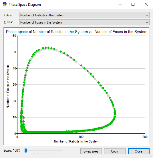
It is possible to swap axes, copy the plot, or focus on its part. Dimmed arcs show the direction of the development of the system as time progresses.
Transparent mode
By default, the node property sheets are displayed in opaque mode, i.e., when open, they cover whatever is under them. Here is a screen shot from the Hepar II model
It is possible to make the property sheets transparent, which may be handy when navigating through a model. Transparent mode allows to see what is under the property sheets. The same model in transparent mode looks as follows
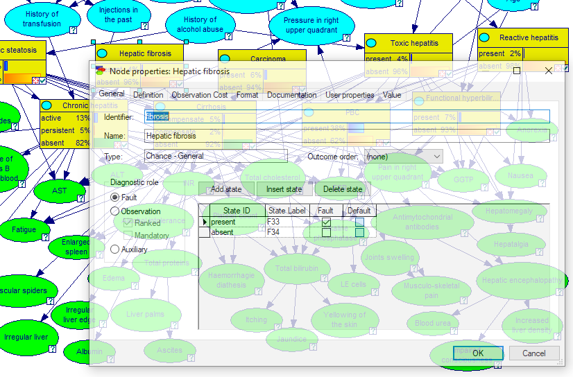
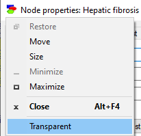
To toggle between the opaque and transparent mode, check the Transparent flag in the System Menu, available by clicking on the icon in the upper-left corner of the node property sheets
The setting holds only for the currently open property sheet and only as long as it is open.
The transparent mode may be especially useful when the property sheets are maximized, in which case it allows to see what else is on the screen and in the Graph View window.