Similarly to hybrid static Bayesian networks, it is possible to create hybrid DBNs, i.e. DBNs that contain both discrete and continuous nodes. This is a powerful modeling mechanism that makes it possible to mimic models based on difference equations (difference rather than differential equations because time in DBNs as we know them is discrete). Consider the well known predator-prey model introduced and studied theoretically by Alfred J. Lotka and later by Vito Volterra (see https://en.wikipedia.org/wiki/Lotka%E2%80%93Volterra_equations for more information). The model is based on two differential equations that describe how the population of prey and the population of predators depend on each other:
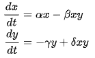
where x is the population density of prey, y is the population density of predators, t represents time, and α, β, γ, and δ represent other model parameters, such as growth and death rates and the effect of presence of prey on predators on each other.
Let us model rabbits (R) as prey and foxes (F) as predators. We transform the Lotka-Volterra differential equations to the two following difference equations:
R{t+1} - R{t} = α*R{t} - β*R{t}*F{t}
F{t+1} - F{t} = - γ*F{t} + δ*R{t}*F{t}
and construct variables R and F in the temporal plate. Given the presence of a differences between time t and time t+1, we need to specify the initial conditions for each of the variables, i.e., their values at t=0. Let us define R{0} and F{0} as small numbers coming from the Uniform(5,15) distribution. We can add noise to the equations, for example as a small number derived from the Normal distribution, Normal(0,σ). Because the primary inference technique in our model is simulation, we need to make sure that none of the two variables (R and F) will ever be smaller than zero by means of the Max() function. The effective definitions of each of the two variables in the model under construction will be:
Rabbits:
R{0}=Uniform(5,15)
R{t+1}=Max(R{t}+α*R{t}-β*R{t}*F{t}+Normal(0,σ),0.1)
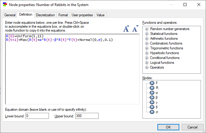
Foxes:
F{0}=Uniform(5,15)
F{t+1}=Max(F{t}+δ*R{t}*F{t}-γ*F{t}+Normal(0,σ),1)

The general rules for writing difference equations in node definitions are as follows.
Definition of a continuous node that is placed in the temporal plate consists of one or more equations. Similarly to what happens in static models involving continuous/equation nodes, it is not necessary to draw arcs between nodes before writing the equations - GeNIe will add arcs automatically as needed.
Writing a single equation that does not involve any temporal influences, e.g., X=Y+2*Z+Q, implies only static links from nodes Y, Z and Q, which can be located either on the temporal plate or outside it.
Temporal equations as above are essentially difference equations. Because a system of difference equations requires a set of initial conditions, a continuous/equation node with temporal influences has to have at least two equations in its definition: one difference equation and at least one equation (in case of a first order difference equation) describing the initial condition, i.e., the value of the variable at the initial time steps that are not described in the highest order difference equation included in the definition. A node that is defined by a single equation may not include temporal influences, so an equation Total{t}=R{t}+F{t} is illegal and should rather take the form of Total=R+F.
Temporal influences are indicated by curly brackets ({ and }) and expressions referring to time steps inside them. When writing a temporal equation, one has to introduce a time variable, which is an arbitrary local identifier that is unique in the model. For example, the equation for the number of rabbits, R{t+1}=R{t}+α*R{t}-β*R{t}*F{t}, uses a local unique identifier t to represent time step. This equation can be rewritten as R{i+1}=R{i}+α*R{i}-β*R{i}*F{i}, without any loss of generality, as long as i is also a unique variable identifier in the model. Both t and i can be used in the same context in other variables, as they have only local scope. The time step identifier used between the curly braces can be also used outside of the braces, in which case it denotes the current time step (time steps is an integer number starting with zero and ending with the total number of steps, as specified in the model). For example, we could extend the rabbits equation by adding Normal noise that increases with the number of steps, e.g., R{t+1}=R{t}+α*R{t}-β*R{t}*F{t}+Normal(0,t/10).
Similarly to discrete DBNs, inference with continuous/equation nodes relies on "unrolling" the model. During unroll operation, the R in the first slice will be initialized with the R{0} equation. All subsequent copies of R in the slices 1, 2, ... will use the second equation. For the 5th slice, for example, the R equation will be rewritten as R_5=R_4+α*R_4-β*R_4*F_4. There is no theoretical upper limit on the number of equations in the temporal equation set of a node, as the number depends on the time order of the equation. For example, to properly define initial conditions when dealing with a third order difference equation, we may require three steps instead of just one:
X{0]=Normal(0,1)+2*Y
X{1}=X{0}+M{0}+N{0}
X{2}=2*X{1}+Uniform(3,4)
X{t+3}=X{t}+5*X{t+1}+Normal(X{t+2},1)+Y
There is a considerable flexibility in how the time order is referred to in difference equations. For example, the last equation can be rewritten with X{t} on the left hand side. The subscript expressions on the right hand side will require adjustments to ensure the difference between the time order of the left hand side and the right hand side remains equal to three. The following three equations are thus equivalent:
X{t+3}=X{t}+5*X{t+1}+Normal(X{t+2},1)+Y
X{t}=X{t-3}+5*X{t-2}+Normal(X{t-1},1)+Y
X{t+1}=X{t-2}+5*X{t-1}+Normal(X{t},1)+Y
The choice of notation does not influence the unroll operation and the solution. The resulting static equations present in the unrolled network will be identical.
With multiple initial conditions, only the equation describing the variable at time step zero requires to use a constant in the left hand side braces. If the node is defined by a single temporal equation between steps 1 and 2, and its final equation requires 3 previous steps as inputs, the equation set could consist of more than one difference equations, e.g.,
X{0}=Normal(0,1)+Y
X{t+1}=X{t}+3*Z{t}
X{t+3}=X{t}+2*X{t+1}+3*X{t+2}+4*Z{t+3}
After the unroll operation, X will be defined for steps 0 through 4 by the following equations
0: X=Normal(0,1)+Y
1: X_1=X+3*Z
2: X_2=X_1+3*Z_1
3: X_3=X+2*X_1+3*X_2+4*Z_3
4: X_4=X_1+2*X_2+3*X_3+4*Z_4
Note that for backward compatibility we keep the original node identifier in the slice zero, so there is no X_0 but rather X is used instead.
We add the model parameters as static variables outside of the temporal plate (α, β, γ, δ and σ) and set them to 0.1, 0.01, 0.3, 0.005 and 0 respectively. We set the number of time steps to 300 and we also set the initial (t=0) number of rabbits and foxes at 10 each. The complete model (available as an example model Foxes Rabbits Hybrid.xdsl) looks as follows
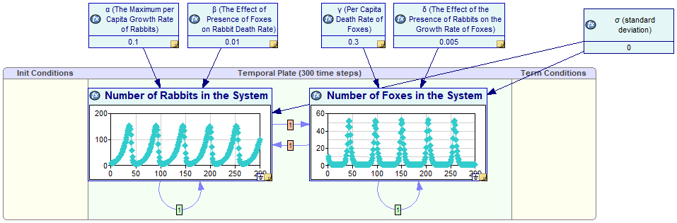
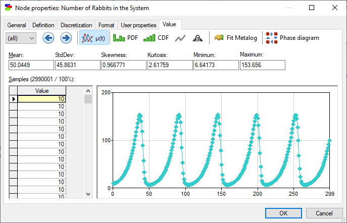
The model is capable of deriving the number of foxes and rabbits as a function of time, as shown in the screen shot above. The Value tab of R shows the solution of this model, the number of rabbits as a function of time.
The Value tab of F shows the number of foxes as a function of time.
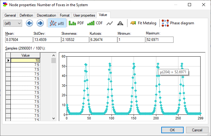
The model allows for deriving so-called phase-space diagrams, which are plots of the value of one variable as a function of another, in this case the number of foxes in the system as a function of the number of rabbits in the system. Pressing the Phase diagram (![]() ) button invokes the following dialog
) button invokes the following dialog
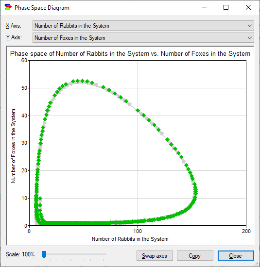
The greatest advantage of a Dynamic Bayesian network model over a system of differential/difference equations is that solving the former is based on stochastic simulations rather than an analytical solution. This allows for modeling that is not constrained by what is solvable but rather focusing on the subject matter and the theoretical and practical aspects of the problem at hand. In addition to that, DBNs allow for injecting uncertainty into models and processing this uncertainty correctly. It also allows for entering observations at different time steps. The above plots are based on observing that there are 10 rabbits and 10 foxes at time zero.