Inference in a DBN, similarly to inference in a BN, amounts to calculating the impact of observation of some of its variables on the probability distribution over other variables. The additional complication is that both evidence and the posterior probability distributions are indexed by time. We will go through the example used in the previous sections to demonstrate setting evidence, running an algorithm, and viewing the results.
Setting temporal evidence
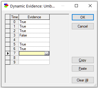
Suppose that during her week-long shift, the guard observes an umbrella on every day except for day three (day count starts with zero), when she was sure she did not see any umbrella and day four, when she forgot whether she saw an umbrella or not. This means that the evidence vector for the node Umbrella is as follows:
Umbrella[0:6]= [true, true, true, false, --, true, true].
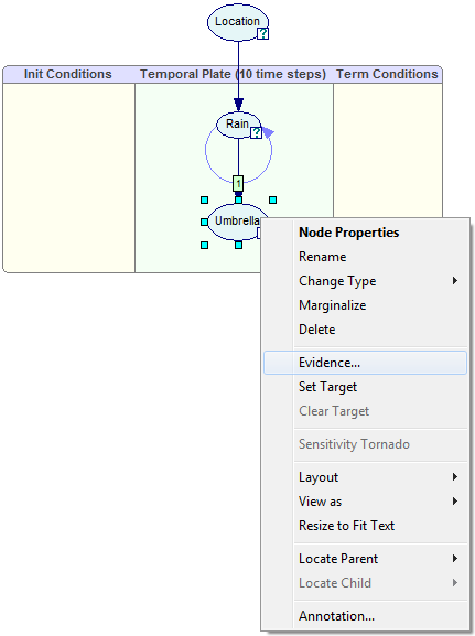
To enter this evidence, we right-click on the Umbrella node and select Evidence...
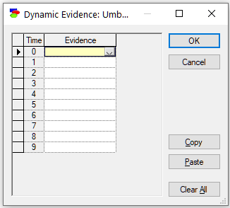
This invokes the Dynamic Evidence dialog
We enter the evidence vector as specified above:
Running the belief updating algorithm
Running the belief updating algorithm is identical to doing so in Bayesian networks. We press the Update (![]() ) button or select Update Beliefs from the Network Menu. GeNIe converts the DBN into a Bayesian network (this is called unrolling - see below) and updates the beliefs using the selected belief updating algorithm.
) button or select Update Beliefs from the Network Menu. GeNIe converts the DBN into a Bayesian network (this is called unrolling - see below) and updates the beliefs using the selected belief updating algorithm.
Viewing the results in discrete DBN nodes: Temporal posterior beliefs
After the network has been updated, we can view its temporal beliefs, which are marginal posterior probability distributions as a function of time. Hovering the mouse over the status icon yields the following views:
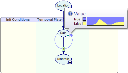
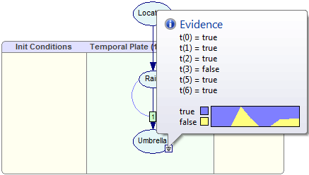
Please note that the Umbrella node is an evidence node. Its temporal beliefs are also well defined, albeit for those time slots for which there are observations, they are constant.
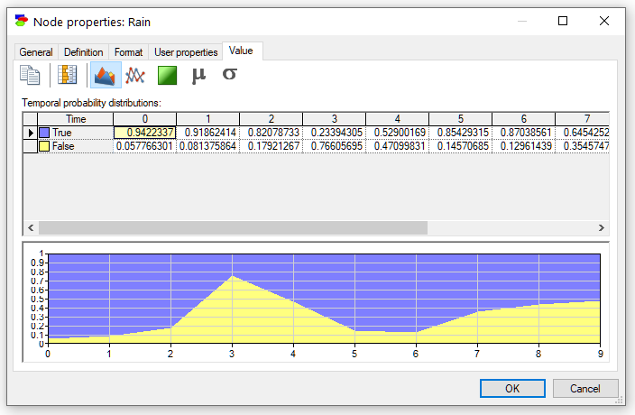
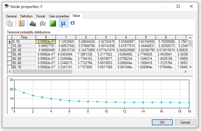
We can view the temporal beliefs in the Value Tab of a node as a spreadsheet indexed by the time steps. Selecting cells in the results spreadsheet and pressing the Copy (![]() ) button copies the cells for use outside of GeNIe.
) button copies the cells for use outside of GeNIe.
In addition to the numerical values of the marginal posterior probabilities over time, we can view the results graphically. Pressing the Area chart (![]() ) button displays the posterior marginal probabilities graphically:
) button displays the posterior marginal probabilities graphically:
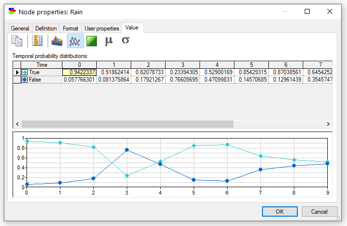
Pressing the Time series (![]() ) button shows the posteriors as a time series plot (a curve for every state of the variable):
) button shows the posteriors as a time series plot (a curve for every state of the variable):
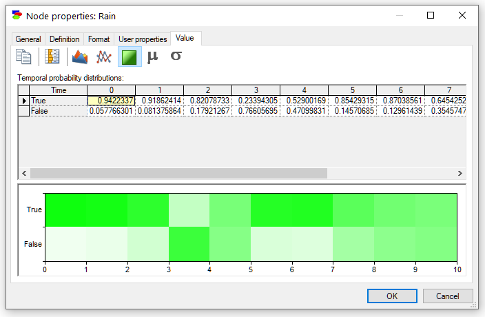
Finally, pressing the Contour plot (![]() ) button displays the posterior marginal beliefs as a contour plot with probabilities displayed by colors. Hovering over individual areas shows the numerical probabilities corresponding to the areas/colors. The Contour plot is especially useful when the variable has many states and shows graphically the weight of probability mass.
) button displays the posterior marginal beliefs as a contour plot with probabilities displayed by colors. Hovering over individual areas shows the numerical probabilities corresponding to the areas/colors. The Contour plot is especially useful when the variable has many states and shows graphically the weight of probability mass.
There is one more plot available in case of discrete numerical variables, notably plot of the mean of the variable as a function of time. To show that plot, please press the Mean button (![]() ).
).
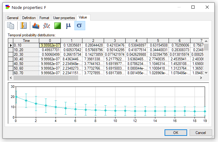
The plot can be enhanced by displaying the standard deviation around the mean. We can accomplish this by pressing the Standard deviation button (![]() )
)
The pictorial representation of the temporal probability distributions can be copied and later pasted into another application for the purpose of documentation or reporting. To copy the pictorial representation of the temporal probability distributions, right-click on it, select Copy, and subsequently choose Paste Special in the destination application.
One should add that the relative size of the table and the plot area can be in each of the above plots adjusted by clicking and dragging on the divider line.
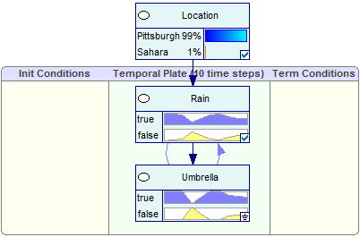
Marginal posterior probabilities can be also shown on the screen permanently by the changing the node view to Bar chart. This can be accomplished by selecting nodes of interest and then changing the view of the nodes through the Node-View as-Bar Chart option.
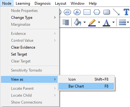
The Bar chart view allows for displaying the temporal posterior marginal probabilities on the screen permanently.
Viewing results: Temporal beliefs
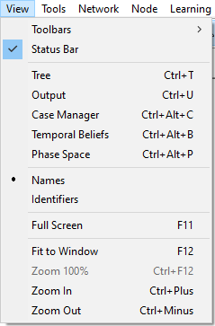
Marginal posterior probabilities can be also shown as a plot in a separate window called Temporal Beliefs. The Temporal Beliefs window can be opened by selecting it on the View menu.
This opens the Temporal Beliefs window with the probability of the Focus node (in our model, it is the node Large Market Share) displayed
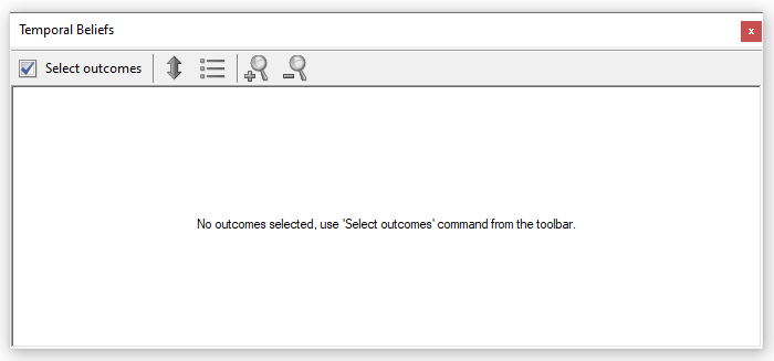
We select outcomes to be displayed by pressing the Select outcomes button.
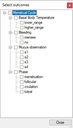
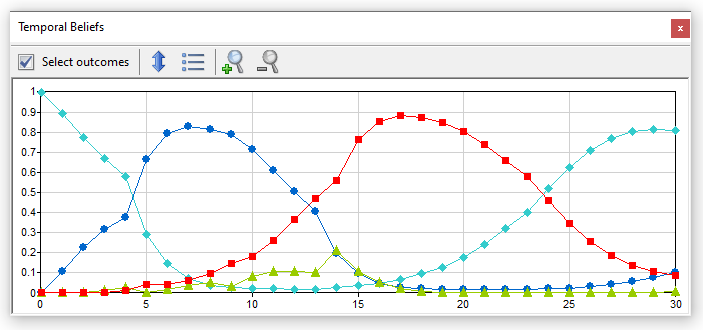
In this model, it is of interest to view the probabilities of various phases of the monthly cycle
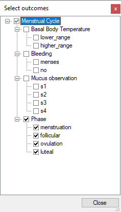
The windows shows the probabilities of the selected outcomes (phases of the monthly cycle) as a function of time
Pressing the Show chart legend (![]() ) button toggles between a plot with or without legend.
) button toggles between a plot with or without legend.
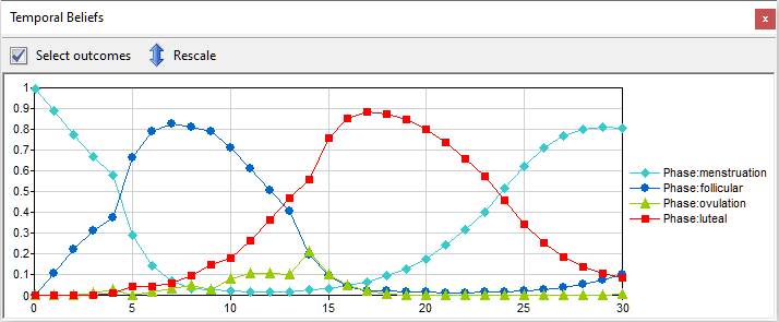
Rescale chart to show only relevant part of [0..1] range (![]() ) button allows for changing the range of the vertical axes from the default [0..1] to a range taken by the most likely outcome shown in the plot. Zoom time in (
) button allows for changing the range of the vertical axes from the default [0..1] to a range taken by the most likely outcome shown in the plot. Zoom time in (![]() ) and Zoom time out (
) and Zoom time out (![]() ) buttons allow for zooming in and out along the horizontal axis.
) buttons allow for zooming in and out along the horizontal axis.
Viewing the results in continuous/equation DBN nodes
After the network has been updated, for each continuous/equation node, we can view their values as a function of time.
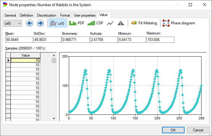
In addition to the mean of the variable as a function of time, we can view the probability distribution over the possible values at each time step. To move across various time steps, please select the desired slice using the Time slice (![]() ) pop-up menu use the Previous time slice (
) pop-up menu use the Previous time slice (![]() ) and Next time slice (
) and Next time slice (![]() ) buttons.
) buttons.
Show sample mean over time (![]() ) button displays the mean of the variable of time (this is the default display). Show probability density function (
) button displays the mean of the variable of time (this is the default display). Show probability density function (![]() ) button shows the histogram of samples, Show cumulative probability function (
) button shows the histogram of samples, Show cumulative probability function (![]() ) button shows the cumulative histogram of samples, Display density function as line chart (
) button shows the cumulative histogram of samples, Display density function as line chart (![]() ) button changes both histograms into lines, Show normal distribution over density function (
) button changes both histograms into lines, Show normal distribution over density function (![]() ) button fits Normal distribution to the sample, and Fit metalog distribution (
) button fits Normal distribution to the sample, and Fit metalog distribution (![]() ) button invokes the Metalog Distribution dialog that allows for fitting a metalog distribution the samples.
) button invokes the Metalog Distribution dialog that allows for fitting a metalog distribution the samples.
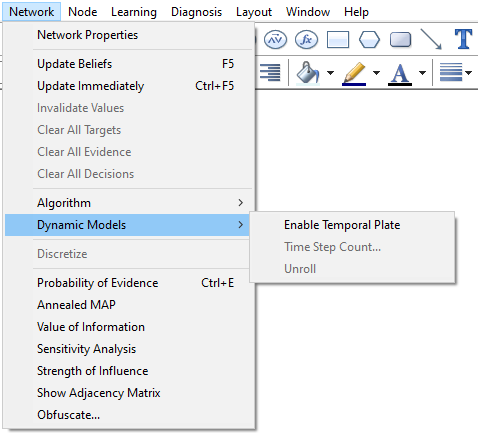
Unrolling the DBN
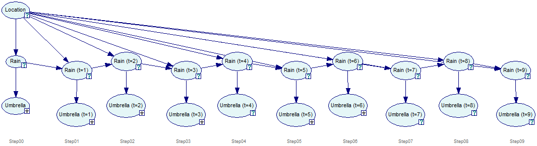
As we mentioned above, for the purpose of inference, GeNIe converts the DBN into a Bayesian network and updates the beliefs using the selected belief updating algorithm. It can be useful, for example for model debugging purposes, to explicitly unroll a temporal network. GeNIe provides this possibility through the Network-Dynamic Models-Unroll option.
GeNIe creates a new network that has the temporal network unrolled for the specified number of time-slices. The unrolled network that is a result from unrolling the temporal network is cleared from any temporal information whatsoever. It can be edited, saved and restored just like any other static network. The screen shot below shows the unrolled network representation of a temporal network and how the original DBN can located back from the unrolled network.
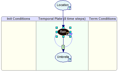
It is possible to locate a node in the temporal network from the unrolled network by right-clicking on the node in the unrolled network and selecting Locate Original in DBN from the context-menu.
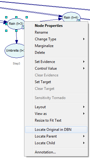
The node will be identified in the original DBN:
DBNs that include continuous/equation nodes are also unrolled for the purpose of inference and can be examined similarly.