The fundamental algorithm used for equation-based (continuous) and hybrid models is stochastic sampling. It is the preferred method when the network does not contain any evidence nodes. With evidence nodes, the situation becomes more complex and there are no universally reliable stochastic sampling algorithms. In all such cases, the algorithm for continuous and hybrid models is based on discretization.
Stochastic sampling algorithms
The reason why stochastic sampling algorithms are fundamental for equation-based models is that GeNIe puts no limitations on the models and, in particular, no limitations on the equations and distributions used in the node definitions. The modeling freedom given by GeNIe comes with a price tag - it prevents us from using any of the approximate schemes developed for special cases of continuous models. We will demonstrate the use of a stochastic sampling algorithm on the simple model used throughout this section.
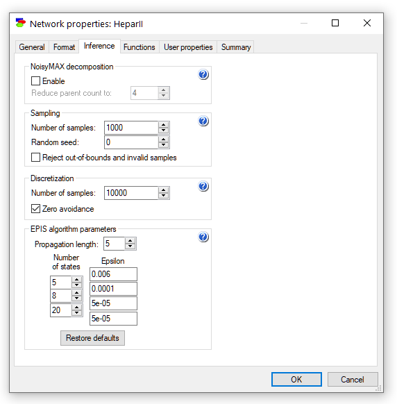
Let us start with setting the number of samples to 1,000,000 from the default 10,000. We can do this in the Sampling pane of the Inference tab of the Network properties. We should generally choose the number of samples to be as large as possible given the constraints on the execution time. Execution time is pretty much linear in the number of samples, so mental calculation of what is admissible is easy. For the model at hand, consisting of only three variables, 1,000,000 will give us high quality results and, at the same time, it will not be noticeable in terms of execution time.
We invoke inference by pressing the Update (![]() ) tool on the Standard Toolbar. Section Viewing results discusses how to view and interpret the results of the algorithm.
) tool on the Standard Toolbar. Section Viewing results discusses how to view and interpret the results of the algorithm.
Auto-discretization
When a continuous or hybrid network contains evidence that is outside of the root (parent-less) nodes, there are no universally applicable stochastic sampling algorithms. GeNIe relies in all such cases on an algorithm that we call auto-discretization.
The algorithm translates the original continuous, equation-based network into a discrete Bayesian network. No changes are made to the original network definition but inference is performed in a temporary discrete Bayesian network, created solely for the purpose of inference. Subsequently, inference results are copied back to the original model. Conditional probability tables generated for the purpose of inference are of transient nature - they are derived for the purpose of inference and they are not saved with the model.
In order to use this algorithm, the user needs to enhance the definitions of the nodes in the network with a specification of the on-demand discretization. If this is not done, GeNIe, in the spirit of preserving the syntactical correctness of every model, will discretize every variable into two states and will place a message "Equation node <node name> was discretized." in the Output window. This, in most cases, is insufficient to obtain any insight and we advise to revisit the nodes in question in order to discretize them into more intervals. Generally, the more discretization intervals have been specified, the more precise the calculation. Please do keep in mind that many discretization intervals will increase the complexity of inference.
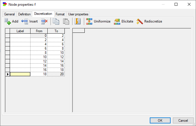
In our example, we start with the node f
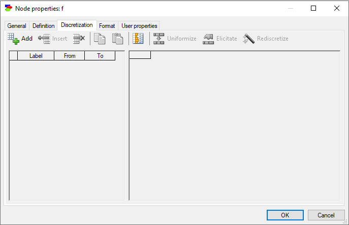
The three buttons in the top-left, Add, Insert, and Delete serve a similar purpose to the corresponding buttons in the Definition tab of discrete nodes. We add 10 intervals using the Add interval (![]() ) button
) button
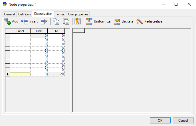
and subsequently press Uniformize (![]() ) button.
) button.
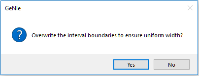
Pressing Yes creates new boundaries for the intervals and results in the following discretization
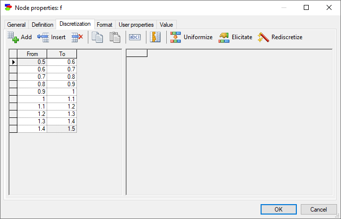
In case of continuous/equation nodes, it is best to leave labels empty, as this forces GeNIe to display ranges of inetervals rather than text labels. However, should the user prefer to add labels to intervals, this can be accomplished by pressing the Show interval labels (![]() ) button, which causes GeNIe to show (default) or hide the interval labels. The following screen shot shows the dialog with the interval labels hidden.
) button, which causes GeNIe to show (default) or hide the interval labels. The following screen shot shows the dialog with the interval labels hidden.
At this point, we have two choices: Elicitation or automatic derivation of the discrete distribution over the intervals from the continuous definition of the node. Pressing the Rediscretize (![]() ) button derives the probabilities from the definition of the node using stochastic sampling. The number of samples generated for the purpose of discretization is specified in the Network properties, Inference tab.
) button derives the probabilities from the definition of the node using stochastic sampling. The number of samples generated for the purpose of discretization is specified in the Network properties, Inference tab.
In addition to the Number of discretization samples, which determines the number of samples used in deriving the conditional probability tables in auto-discretized models, the tab allows the user to avoid zero probabilities in discretized conditional probability distributions. This option works only in chance nodes, i.e., nodes that contain reference to noise (expressed as calls to random number generator functions). Zeros in probability distributions lead to potential theoretical problems and should be used carefully, only if we know for sure that the probability should be zero. Once a zero, a probability cannot be changed, no matter how strong the evidence against it. We recommend (Onisko & Druzdzel, 2012) for a discussion of practical implications of this problem.
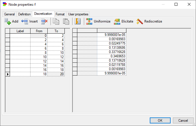
Rediscretization of the node f with 10,000 samples and zero avoidance should lead to the following discretized definition.
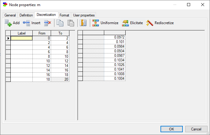
We repeat the same process for the variable m with also 10 intervals.
And for the variable a with 10 intervals.
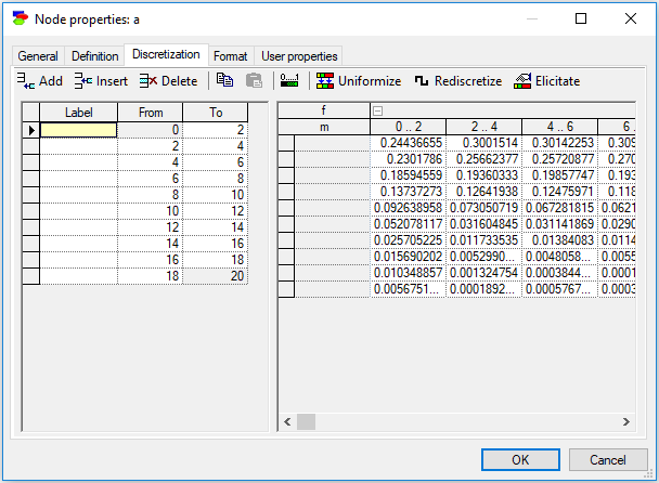
Please note that the CPT for node a is very large and contains 10x10=100 distributions, one for each combination of discretized values of the variables f and m. The screen shot above shows only its fragment.
Pressing Elicitate (![]() ) button shows the node's CPT and allows us to adjust the discretization boundaries manually.
) button shows the node's CPT and allows us to adjust the discretization boundaries manually.
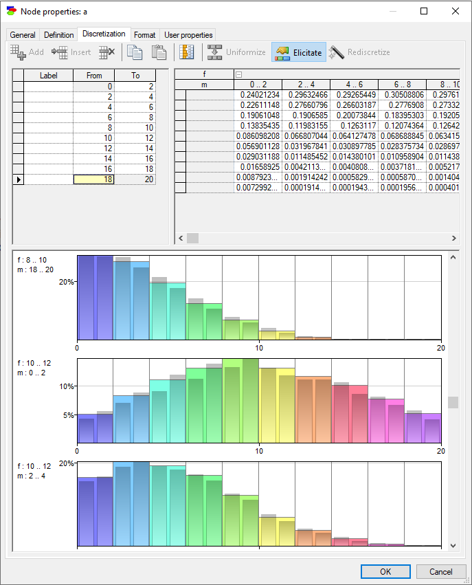
Similarly to the histogram dialog in Cleaning Data section, you can adjust the boundaries of the discretization intervals manually by dragging the vertical lines that separate the samples towards right and left and observing how this impacts each of the conditional probability tables for the node (you can see each of the 100 conditional probability distributions by scrolling the dialog). The conditional probability tables are pictured as histograms of discretization samples.
The discretization is all we need to run the auto-discretization algorithm. We run the algorithm by pressing the Update (![]() ) tool on the Standard Toolbar.
) tool on the Standard Toolbar.
One last remark that we would like to include in this section is that discretization is a powerful tool for constructing Conditional Probability Tables (CPTs). If we understand a part of the modeled system well enough to capture the interactions among some of its variables by means of equations, we can use discretization to derive conditional probability tables. Once a table has been constructed, we can copy it and paste it into a discrete node.