Network properties sheet summarizes all properties that are specified at the network level. It can be invoked in three ways:
1.Double clicking on a clear area of the network in the graph view.
2.Right clicking on the name of the network in the Tree View or right clicking on a clear area of the network in the Graph View. This will display the Network Pop-up menu. Select Network Properties from the menu.
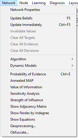
3.Select Network Properties from the Network Menu as shown below.
The Network properties sheet, once opened, consists of several tabs.
Shown below is a typical Network Properties Sheet with the General tab:
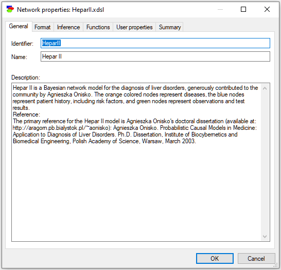
General tab
The General tab of Network properties (shown above) consists of the following fields:
Identifier displays the identifier for the network, which is user-specified. Identifiers must start with a letter, and can contain letters, digits, and underscore (_) characters. The identifier for the network shown above is HeparII.
Name displays the name for the network, which is user-specified. There are no limitations on the characters that can be part of the name. The name for the network shown above is Hepar II.
Description is a free text describing the network. Please note that a model is a documentation of the problem and use descriptions generously.
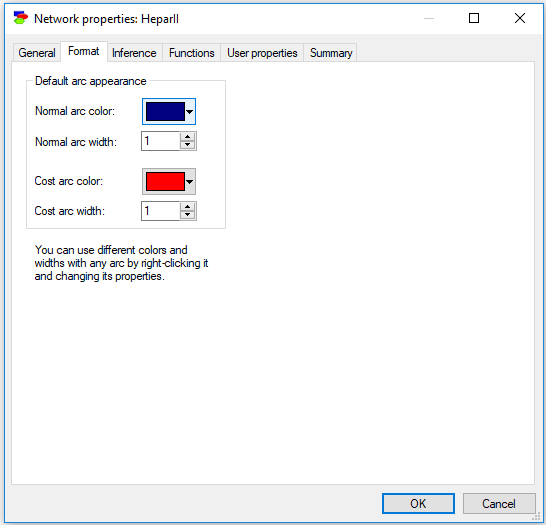
Format tab
The Format tab of Network properties (shown below) allows for choosing the default appearance of arcs in the network. These defaults can be overridden in each individual model arc.
Inference tab
The Inference tab allows the user to set the various parameters of GeNIe inference algorithms.
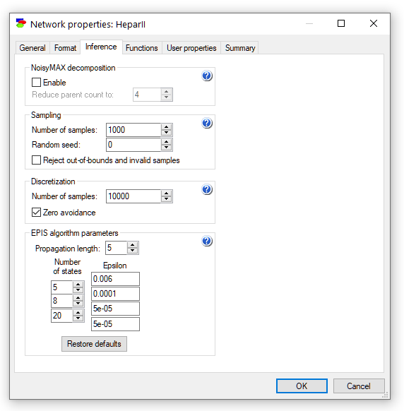
The Inference tab allows you to enable Noisy-MAX decomposition, which makes inference in models with Noisy-MAX nodes more efficient and, in very complex models, even possible at all. The Reduce parent count to parameter controls the decomposition of Noisy-MAX models. After the decomposition, no Noisy-MAX node will have more than that number of parents. The default value of 4 is reasonable but if inference is slow on your network, you may want to explore other values.
Number of samples sets the number of samples used in each execution of a sampling algorithm. All sampling algorithms are approximate. The number of samples determines the precision of the results (the more samples, the more precise the result, although no simple formula exists that translates the number of samples into precision) but at the same time it determines the computation time (the more samples, the longer the running time - running time is pretty much linear in the number of samples). Error in the posterior marginal probabilities calculated by the EPIS-BN algorithm reduces as a square root of the number of samples. Please keep in mind that if you would like to recompute the values with the new number of samples (larger number of samples give you a higher precision), you will need to invoke the updating algorithm again, either by pressing the Update tool (![]() ) or, when Update immediately option is on, by invalidating all values (see the Invalidate values command) and by this forcing GeNIe to recompute them during the next run of the algorithm.
) or, when Update immediately option is on, by invalidating all values (see the Invalidate values command) and by this forcing GeNIe to recompute them during the next run of the algorithm.
Random seed allows for making stochastic sampling algorithms (such as AIS-BN or EPIS-BN) to be replicable, i.e., to produce the same results each time they are run in a give situation (i.e., with the same model and the same set of observations). Any number that is different than zero makes the results replicable. A random seed of zero uses a truly random number seed and makes the results different each time the algorithm is run. This value is a property of the model and is saved in the .xdsl file.
Reject out-of-bound and invalid samples option, when checked, causes every sample that is invalid (e.g., not a number when the algorithm encounters division by zero or square root of a negative number) or out of bounds (defined on the Definition tab of the Node properties) to be discarded. Having this option checked improves the convergence of the algorithm at the expense of computation time. Outlier samples make minimal contribution to the posterior probability distribution in importance sampling, while costing as much as all other samples in computation.
Discretization pane serves to set the number of samples in deriving the CPTs for discretized continuous nodes (see also the Autodiscretization algorithm). Higher number of samples takes more time but leads to a better precision of parameters. Zero avoidance, when checked, avoids placing zeros in the CPTs, even if there are no samples generated for a given parameter.
EPIS algorithm parameters are used to fine tune the EPIS algorithm execution. The EPIS algorithm uses Loopy Belief Propagation (LBP), an algorithm proposed originally by Judea Pearl (1988) for polytrees and later applied by others to multiply-connected Bayesian networks. EPIS uses LBP to pre-compute the sampling distribution for its importance sampling phase. Propagation length is the number of LBP iterations in this pre-computation. EPIS uses Epsilon-cutoff heuristic (Cheng & Druzdzel, 2000) to modify the sampling distribution, replacing probabilities smaller than epsilon by epsilon. The table in the Sampling tab allows for specifying different threshold values for nodes with different number of outcomes. For more details on the parameters and how they influence the convergence of the EPI-BN algorithm, please see (Yuan & Druzdzel 2003).
Functions tab
The Functions tab allows the user to define functions that will be used in the model. The following sheet contains three definitions of functions: o2p(), p2o(), and tang(). GeNIe functions may not be recursive but they may refer to functions defined earlier (in the same Functions tab).
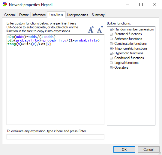
It is possible to test the newly defined functions by evaluating calls to them with concrete values of parameters at the bottom of the tab. Please note that arguments of the evaluated function have to be constants.
User-defined functions (also called Custom functions) are defined per network and stored along with the network. GeNIe copies user-defined functions between networks when nodes using them are copied from a source network and pasted in the destination network. In this case, conflicts may occur, for example a function with the same definition may exist already in the destination network. GeNIe performs a simple check of the name of the function, its number of parameters, and determinism status (i.e., whether the function makes calls to random number generators) and will use the definition in the destination network if these three agree. Otherwise, it will copy the definition from the source to the destination network. We recommend that meaningful names are used and different definitions of the same function in different models are avoided.
User properties tab
User properties tab allows the user to define properties of the model that can be later retrieved by an application program using SMILE.
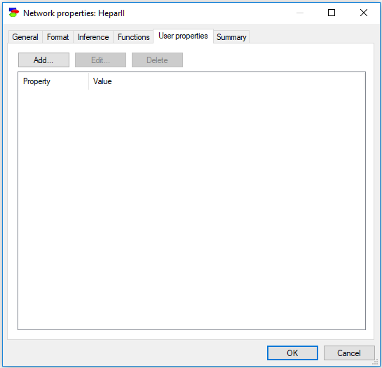
For example, we can add a property AUTHOR with the value "https://www.bayesfusion.com/". Neither GeNIe nor SMILE use these properties and they provide only placeholders for them. They are under full control and responsibility of the user and/or the application program using the model. GeNIe and SMILE support only editing and storing/retrieving them.
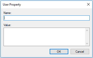
Button Add invokes the following dialog that allows for defining a new user property:
Buttons Edit and Delete allows for editing and removing a selected property, respectively.
Summary tab
Summary tab contains summery statistics of the network, as illustrated below:
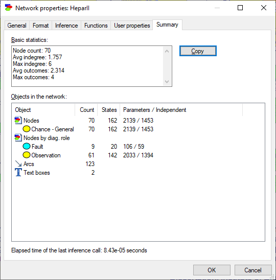
Statistics focus on the structural properties of the network, such as the number of nodes of each type in the network, the average and the maximum in-degree (the number of parents of a node), the average and the maximum number of outcomes of nodes, node counts by their diagnostic role, the number of arcs and the number of text boxes, and, finally, the number of states and parameters. Independent parameters take into account that some parameters are just complements, making sure that probabilities have to add up to 1.0. Hepar II, shown in all illustrations in this section, contains 70 nodes, of which 9 are diagnostic fault nodes (diseases) and 61 are observation nodes. The number of arcs (123) and the average in-degree (1.757) give an idea of the structural complexity of the network. Elapsed time of the last inference call gives an idea of the difficulty that your computer system experienced with solving the model.