An crucial element of learning is validation of the results. We will show it on an example data set and a Bayesian network model learned from this data set.
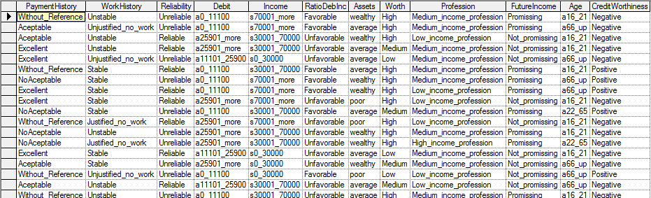
Suppose we have a file Credit10K.csv consisting of 10,000 records of customers collected at a bank. Each of these customers was measured on several variables, Payment History, Work History, Reliability, Debit, Income, Ratio of Debts to Income, Assets, Worth, Profession, Future Income, Age and Credit Worthiness. The first few records of the file (included among the example files with GeNIe distribution) look as follows in GeNIe:
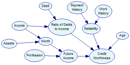
Supposed we have learned or otherwise constructed a Bayesian network model that aims at capturing the joint probability distribution over these variables. The main purpose of constructing this model is to be able to predict Credit Worthiness of a new customer applying for credit. If this customer comes from the same population as previous customers, we should be able to estimate the probability of Positive Credit Worthiness based on the new customer's characteristics. Let the following be the model (it is actually model Credit.xdsl, available among the example models):
Running validation
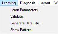
We can perform evaluation of the model by choosing Validate... from the Learning menu
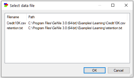
If only one model and one data file are open, it is clear that we want to evaluate the model with the data file. If there are more than one data file open in GeNIe, the following dialog pops up
After selecting the file Credit10K.csv, we proceed with the following (Match Network and Data) dialog, whose only function is to make sure that the variables and states in the model (left column) are mapped precisely to the variables defined in the data set (right column). This dialog is identical to the dialog appearing when learning model parameters from data.
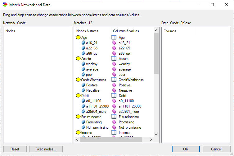
Both lists of variables are sorted alphabetically. The Match Network and Data dialog does text pre-matching and places in the central column all those variables and their states that match (have identical or close to identical names - GeNIe is rather tolerant in this respect and, for example, ignores spaces and special characters). If there is any disparity between them, GeNIe highlights the differences by means of a yellow background, which makes it easy to identify disparities. Manual matching between variables in the model and the data is performed by dragging and dropping. To indicate that a variable in the model is the same as a variable in the data, simply drag-and-drop the variables from one to the other column.
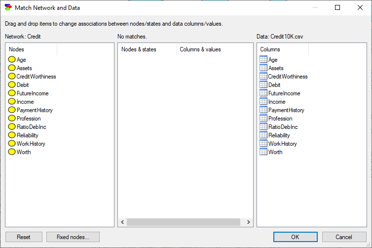
To start the matching process from scratch, use the Reset button, which will result in the following matching:
Fixed nodes... button invokes a dialog that allows for excluding nodes from the learning process in cross-validation
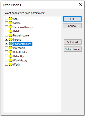
Nodes selected in this dialog (in the dialog above, nodes Income and PaymentHistory) will not be modified by the learning stages of cross-validation and will preserve their original CPTs for the testing phase.
Once you have verified that the model and the data are matched correctly, press OK, which will bring up the following dialog:
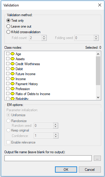
There are two important elements in this dialog.
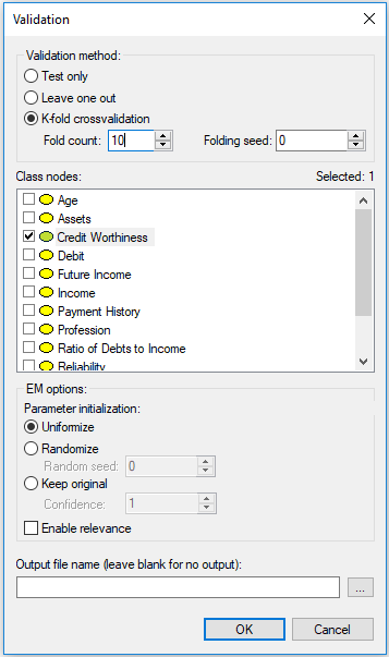
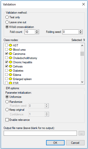
The first element is Validation method. The simplest evaluation is Test only, which amounts to testing the model on the data file. This is suitable to situations when the model has been developed based on expert knowledge or when the model was learned from a different data set and we want to test it on data that it has never seen (e.g., a holdout data set). More typically, we want to both learn and evaluate the model on the same data set. In this case, the most appropriate model evaluation method is cross-validation, which divides the data into training and testing subsets. GeNIe implements the most powerful cross-validation method, known as K-fold crossvalidation, which divides the data set into K parts of equal size, trains the network on K-1 parts, and tests it on the last, Kth part. The process is repeated K times, with a different part of the data being selected for testing. Fold count allows for setting the number of folds. Folding seed is used in setting up random assignment of records to different folds. Setting the Folding seed to anything different than zero (the default) allows for making the process of evaluation repeatable. Zero Folding seed amounts to taking the actual random number seed from the system clock and is, therefore, truly random. The Leave one out (LOO) method is an extreme case of K-fold crossvalidation, in which K is equal to the number of records (n) in the data set. In LOO, the network is trained on n-1 records and tested on the remaining one record. The process is repeated n times. We advise to use the LOO method, as the most efficient evaluation method, whenever it is feasible in terms of computation time. Its only disadvantage is that it may take long when the model is complex and the number of records in the data set is very large. Let us select K-fold crossvalidation with K=10 for our example. Once we have selected a cross-validation technique, EM options become active. The model evaluation technique implemented in GeNIe keeps the model structure fixed and re-learns the model parameters during each of the folds. The default EM options are suitable for this process. Should you wish to explore different settings, please see the description of EM options in the Learning parameters section.
The second important element in the dialog is selection of the Class nodes, which are nodes that the model aims at predicting. At least one of the model variables has to be selected. In our example, we will select Credit Worthiness.
It is possible to produce an output file during the validation process. The output file is an exact copy of the data file with columns attached at the end that contain the probabilities of all outcomes of all class nodes. This may prove useful in case you want to explore different measures of performance, outside of those offered by GeNIe. If you leave the Output file name blank, no output file will be generated.
Here is the Validation dialog again with the settings that we recommend for our example:
Pressing OK starts the validation process. We can observe the progress of the process in the following dialog:

Should the validation take more time than planned for, you can always Cancel it and restart it with fewer folds.
Validation results for a single class node
Accuracy
When finished has finished, the following dialog appears:
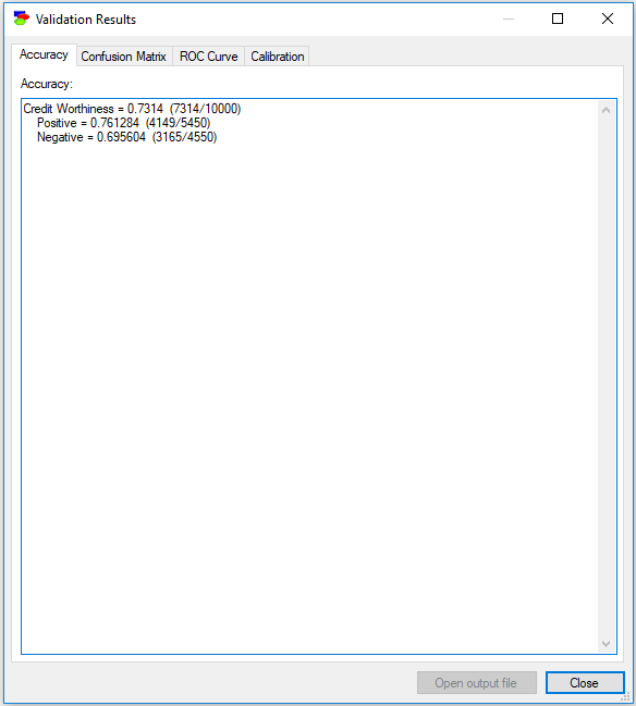
The first tab, Accuracy, shows the accuracy that the model has achieved during the validation. In this case, the mode achieved 73.14% accuracy in predicting the correct Credit Worthiness - it guessed correctly 7,314 out of the total of 10,000 records. It is important to know that during the process, GeNIe chooses for each record the state of the class node that is most probable over all other states. The tab also shows sensitivity and specificity of the model, although it is up to the user to name them. Sensitivity of the model in detecting the Positive Credit Worthiness is roughly 76.13% (4,149 records out of all 5,450 records for which the Credit Worthiness was Positive), with specificity of roughly 69.56% (3,165 records out of all 4,550 records for which the Credit Worthiness was Negative). One could look at this result as showing 69.56% sensitivity and 76.13% specificity in detecting Negative Credit Worthiness.
CTRL-A will select the entire contents of the tab, possibly to be pasted in an editor.
Confusion Matrix
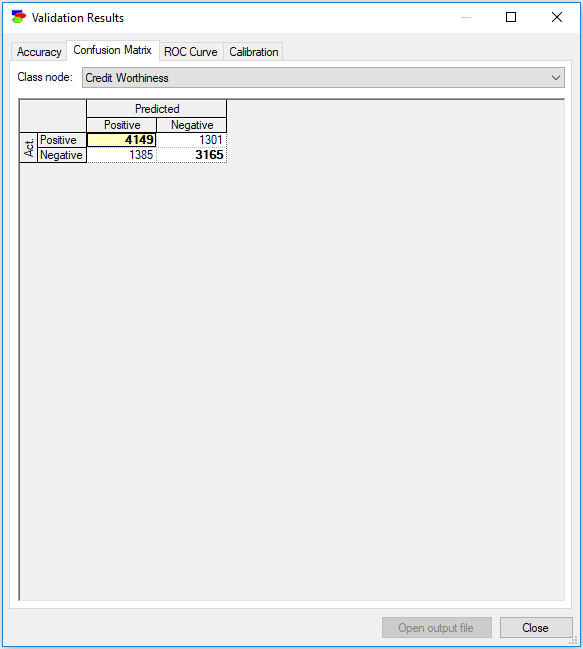
The Confusion Matrix tab shows the same result in terms of the number of records correctly and incorrectly classified. Here the rows denote the actual state of affairs and the columns the model's guess. The diagonal of the confusion matrix (marked by bold numbers) shows the numbers of correctly identified instances for each of the classes. Off-diagonal cells show incorrectly identified classes.
You can copy the contents of the confusion matrix by right-clicking Copy on the selected cells (or right-clicking and choosing Select All). You can paste the selected contents into other programs.
ROC Curve
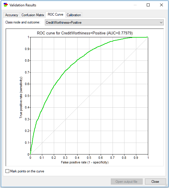
The ROC Curve tab shows the Receiver Operating Characteristic (ROC) curves for each of the states of each of the class variables. ROC curves originate from Information Theory and are an excellent way of expressing the quality of a model independent of the classification decision (in case of GeNIe validation, this decision is based on the most likely state, which in case of a binary variable like Credit Worthiness amounts to a probability threshold of 0.5). The ROC curve is capable of showing the possible accuracy ranges, and the decision criterion applied by GeNIe is just one point on the curve. Choosing a different point will result in a different sensitivity and specificity (and, hence, the overall accuracy). The ROC curve gives insight into how much we have to sacrifice one in order to improve the other and, effectively, helps with choosing a criterion that is suitable for the application at hand. It shows the theoretical limits of accuracy of the model on one plot.
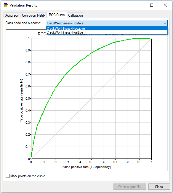
The following ROC curve is for the state Positive of the variable Credit Worthiness. The dim diagonal line shows a baseline ROC curve of a hypothetical classifier that is worthless. A classifier that does its job will have its ROC curve above this diagonal line. Above the curve, we see the Area Under the ROC Curve (AUC) displayed. AUC is a simple, albeit imperfect way of expressing the quality of the model by means of one number.
While AUC gives some ground to comparing accuracies of different models, one has to remember that it loses a lot of information compared to the full ROC curve. Consider two models that classify mushrooms into edible and poisonous. Two models may have similar AUCs but different ROC and the actual shape of the ROC curve may be important. Given the consequences of eating a poisonous mushroom, one should absolutely prefer the model that gives sensitivity 1.0 to poisonous mushrooms the earliest and not necessarily the model that has the highest AUC.
The ROC curve assumes that the class node is binary. When the class node is not binary, GeNIe changes it into a binary node by taking the state of interest (in the ROC curve above, it is the state Positive) and lumping all remaining states into the complement of the chosen state. There are, thus, as many ROC curves for each of the class nodes as there are states. The pop-up menu in the upper-right corner of the dialog allows for choosing a different class variable and a different state. The following screen shot shows the ROC curve for the state Negative of the variable Credit Worthiness.
Finally, the ROC curve is drawn based on a finite number of points, based on the data set used for the purpose of verification. When the number of points is small (typically, this occurs when the data file is small), the curve is somewhat rugged. It may be useful to see these points on the curve. The Mark points on the curve check box turns these points on an off. The following plot shows this idea.
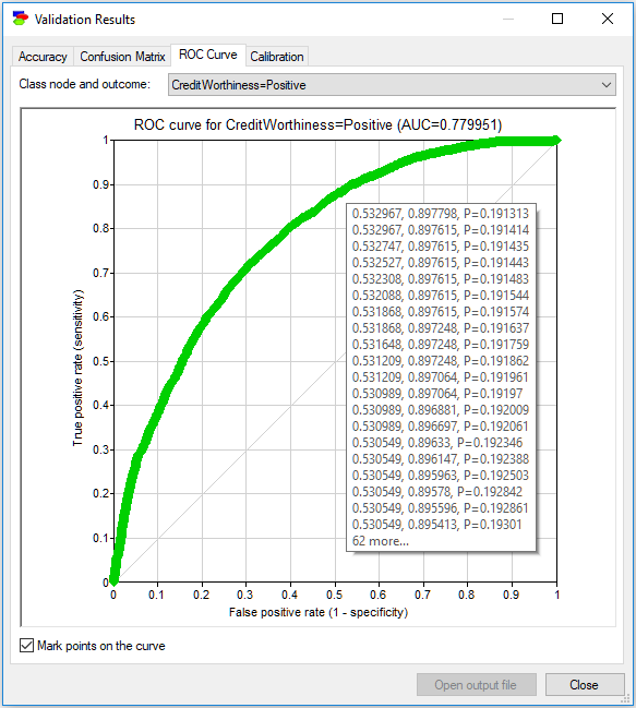
Hovering over any of the points shows the probability threshold value that needs to be used to achieve this point along with the resulting (1-specificity) and sensitivity. In the example above, when the probability threshold is p=0.6, the model achieves sensitivity of 0.7 and specificity of 1-0.237143=0.762857. You can also copy and paste the numbers behind the ROC curve by right-clicking anywhere on the chart, selecting Copy and then pasting the results as text into any text editor (such as Notepad or Word). Pasting into any image editor (or pasting special into a text editor such as Word) results in pasting the image of the ROC curve, in bitmap or picture format, explained in the Graph view section.
ROC calculation is close to issues related to unbalanced classes. By moving on the ROC curve, we change the values of sensitivity and specificity and, in case of probabilistic systems that produce probabilities of various classes, we change the threshold to which we react. One way of handling unbalanced classes in machine learning is oversampling, which is artificially increasing the number of records that belong to the underrepresented classes. We believe that a careful choice of a point on the ROC curve achieves the same.
ROC curve is a fundamental and useful measure of a model's performance. For those users, who are not familiar with the ROC curves and AUC measures, we recommend an excellent article on Wikipedia (https://en.wikipedia.org/wiki/Receiver_operating_characteristic).
Calibration curve
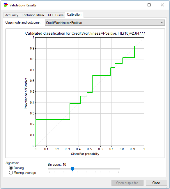
The final tab, Calibration, shows a very important measure of performance of a probabilistic model, notably the calibration curve. Because the output of a probabilistic model is a probability and this probability is useful in decision making, ideally we would like it to be as accurate as possible. One way of measuring the accuracy of a model is comparing the output probability to the actually observed frequencies in the data. The calibration curve shows how these two compare. For each probability p produced by the model (the horizontal axis) for the class variable, the plot shows the actual frequencies in the data (vertical axis) observed for all cases for which the model produced probability p. The dim diagonal line shows the ideal calibration curve, i.e., one in which every probability produced by the classifier is precisely equal to the frequency observed in the data. Because p is a continuous variable, the plot groups the values of probability so that sufficiently many data records are found to estimate the actual frequency in the data for the vertical axis. There are two methods of grouping implemented in GeNIe: Binning and Moving average. Binning works similarly to a histogram - we divide the interval [0..1] into equal size bins. As we change the number of bins, the plot changes as well. It is a good practice to explore several bin sizes to get an idea of the model calibration.
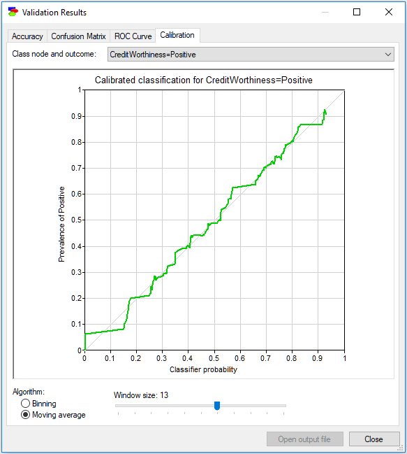
Moving average (see the screen shot below) works somewhat differently. We have a sliding window that takes always the neighboring k output probabilities on the horizontal axis and shows the class frequency among the records in this sliding window on the vertical axis. Here also, as we change the Window size, the plot changes as well. It is a good practice to explore several window sizes to get an idea of the model calibration.
Similarly to the ROC curve, you can copy and paste the coordinates of points on the calibration curve by right-clicking anywhere on the chart, selecting Copy and then pasting the results as text into any text editor (such as Notepad or Word). Pasting into any image editor (or pasting special into a text editor such as Word) results in pasting the image of the calibration curve in bitmap or picture format, explained in the Graph view section.
Validation for multiple class nodes
The above example involved one class node, Credit Worthiness. It happens sometimes that there are several class nodes, for example in multiple disorder diagnosis, when more than one problem can be present at the same time. The Hepar II model (Onisko, 2003) contains nine disorder nodes (Toxic hepatitis, Chronic hepatitis, PBC, Hepatic fibrosis, Hepatic steatosis, Cirrhosis, Functional hyperbilirubinemia, Reactive hepatitis and Carcinoma). When validating the model, we should select all of these.
The results show accuracy for each of the class nodes in separation
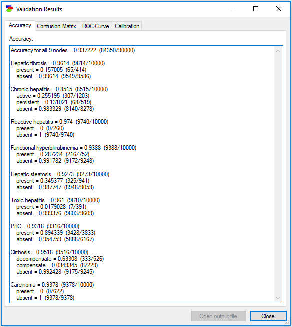
The accuracy tab lists the accuracy for each of the nodes in separation (as opposed to the accuracy in terms of combinations of values of class nodes). Should you wish to calculate the accuracy of the model in pinpointing a combination of values of several nodes, you can always perform a structural extension of the model by creating a deterministic child node of the class nodes in question that has states corresponding to the combinations of interest. Accuracy for those states is equal to the accuracy of the combinations of interest.
It is important to know that when testing a model with multiple class nodes GeNIe never instantiates any of the class nodes. This amounts to observing only non-class nodes and corresponds to the common situation in which we do not know any of the class nodes (e.g., we do not know for sure any of the diseases). Should you wish to calculate the model accuracy for a class node when knowing the value of other class nodes, you will need to run validation separately and select only the class node tested. In this case, GeNIe will use the values of all nodes that are not designated as class nodes.
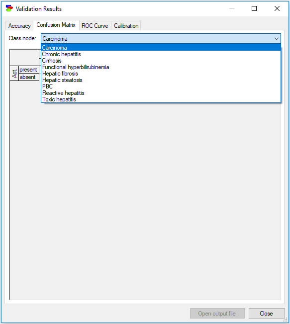
The Confusion Matrix tab requires that you select one of the class nodes - there are as many confusion matrices as there are class nodes.
The remaining two result tabs (ROC Curve and Calibration) require selecting a state of one of the class nodes.
Displaying results based on a validation output file
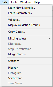
The cross-validation results file contains all the information that are required to show confusion matrix, calculate accuracy, display the ROC and the calibration curves, etc. GeNIe allows for opening an existing validation output file for this purpose. The output data file can be opened exactly the way one opens a data file. Once an output data file is open, please select the Display Validation Results command from the Data Menu.
This will invoke the Validation Results dialog, as described above in this section. No corresponding network needs to be open but the dialog rests on the assumption that the validation output file contains additional columns, as created by GeNIe, i.e., for every class variable X there are corresponding columns X_State1, X_State2, ..., X_StateN, and X_predicted, where State1 through StateN are all states of X. This is precisely what GeNIe places in its output files, so any output file produced by GeNIe is amenable for opening later and displaying validation results.
Log-likelihood calculation
Learning a complete model from data ends with the calculation of the log-likelihood of the data given the model, a measure of the fit of the model to the data. GeNIe allows for calculating the log-likelihood given a model and a data set. To invoke this functionality, please choose Log Likelihood... from the Data menu. Invoking this functionality leads to the dialog that matches the model to the data (making sure that there is a one-to-one correspondence between model variables and their outcomes to columns and their values in the data set). The end result is a number, log-likelihood, which is the logarithm of the probability of the data given the model.
This is always a large negative number (it is the logarithm of a very small probability). Pressing the Copy button copies the number to the clipboard.