The PC structure learning algorithm is one of the earliest and the most popular algorithms, introduced by (Spirtes et al., 1993). It uses independences observed in data (established by means of classical independence tests) to infer the structure that has generated them. Here is the Learn New Network dialog for the PC algorithm:
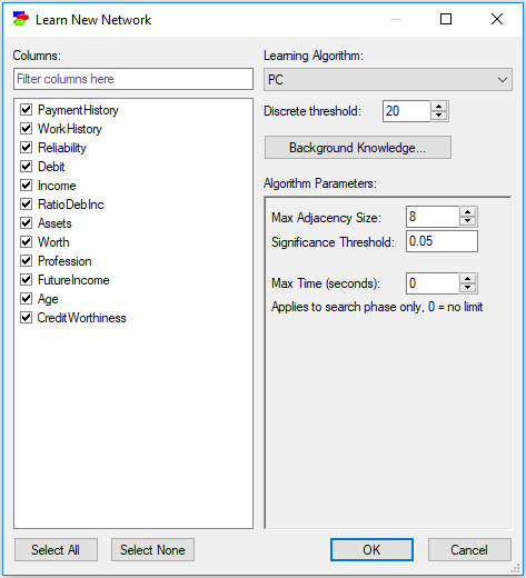
The PC algorithm has three parameters:
•Max Adjacency Size (default 8), which limits the number of neighbors of a node. In practice, this parameter is important for limiting the number of parents that a node corresponding to a variable can have. Because the size of conditional probability tables of a node grow exponentially in the number of the node's parents, it is a good idea to put a limit on the number of parents so that the construction of the network does not exhaust all available computer memory.
•Significance Level (default 0.05) is the alpha value used in classical independence tests on which the PC algorithm rests.
•Max Time (seconds) (default 0, which means no time limit) sets a limit on the search phase of the PC algorithm. It is a good idea to set a limit for any sizable data set so as to have the algorithm terminate within a reasonable amount of time.
Pressing OK and then OK in the Learn New Network dialog starts the algorithm, which ends in the Pattern Editor dialog.
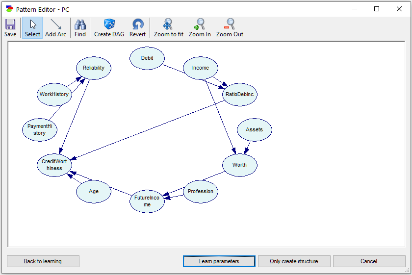
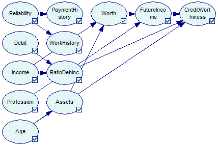
There is one double-edged arc in the pattern (between Assets and Worth). Clicking on the Create DAG (![]() ) button, which picks the direction of each undirected arc randomly to yield an acyclic directed graph, clicking on the Learn parameters button, and then running a graph layout algorithm (Parent Ordering from left to right) results in the following Bayesian network:
) button, which picks the direction of each undirected arc randomly to yield an acyclic directed graph, clicking on the Learn parameters button, and then running a graph layout algorithm (Parent Ordering from left to right) results in the following Bayesian network:
The PC algorithm is the only structure learning algorithm in GeNIe that allows for continuous data. The data have to fulfill reasonably the assumption that they come from multivariate normal distribution. To verify this assumption, please check that histograms of every variable are close to the Normal distribution and that scatter plots of every pair of variables show approximately linear relationships. Voortman & Druzdzel (2008) verified experimentally that the PC algorithm is fairly robust to the assumption of multi-variate Normality.
Let us demonstrate the working of the PC algorithm on a continuous data set retention.txt, included among the example data sets.
Here is the suggested specification of prior knowledge about the interactions among the variables in the data set:
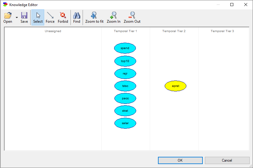
Pressing OK and then OK in the Learn New Network dialog starts the algorithm, which ends in the Pattern Editor dialog.
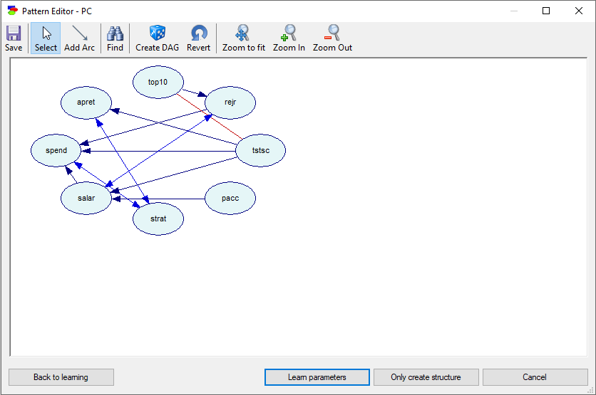
The only two causes of the variable apret (average percentage of student retention) are tstsc (average standardized test scores of incoming students) and strat (student-teacher ratio). The connection between strat and apret disappears when we repeat the learning with the Significance Level parameter set to p=0.01. This example is the subject of a paper by Druzdzel & Glymour (1998), who concluded that the only direct cause of low student retention at US universities is the quality of incoming students. This study is one of the successful examples of causal discovery, and its conclusion was verified empirically later in a real-life experiment by Carnegie Mellon University.
It is a good idea to run the PC algorithm for a range of values of the Significance Threshold parameter. Because PC relies on classical independence tests in which the null hypothesis is "Independence," a low significance threshold makes it harder to reject independence (null hypothesis) and, effectively, the graphs tend to be sparser. A significance threshold that is a very small number may lead to reduction of connectivity by removing weaker connections. Arcs that remain for very small values of the significance threshold may be trusted as fairly robust. When we make the significance threshold very high (0.1 or, for small data sets, even 0.2), the learned graphs are going to be dense (please note that a high significance threshold makes it easy to reject the null hypothesis, i.e., "independence"). Those arcs that are missing can be trusted - even though it was easy to reject independence, it was not rejected.
A word of caution when you use the PC algorithm. The graphs learned by the algorithm tend to be dense. If that happens, reducing the significance threshold parameter may help. It is risky to proceed to learning parameters or even creating a structure without learning parameters when there are nodes in the Pattern Editor that have many parents, as the size of the probability tables may exhaust your computer's memory. Reducing the significance threshold or trying a different algorithm altogether is the simplest way of solving this problem. Also, when you see a graph that may be too complex to be represented in your computer, please do make sure to save your work before proceeding.