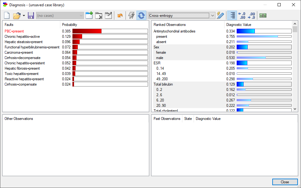
GeNIe and SMILE include three basic measures of diagnostic value of information: (1) Max Probability Change, (2) Cross-entropy, and (3) Normalized Cross-entropy. Each of them produces some insight into the value of observing any of the observation nodes but it is hard to argue for any of them as being the best. We discuss the three measures below in the context of pursuing a single fault. A discussion of how these measures are extended to multiple faults will follow.
Max Probability Change
This measure lists for every state of an observation node the change in the probability of the fault that is being pursued. In the default view, we see for each observation node the maximum probability change.
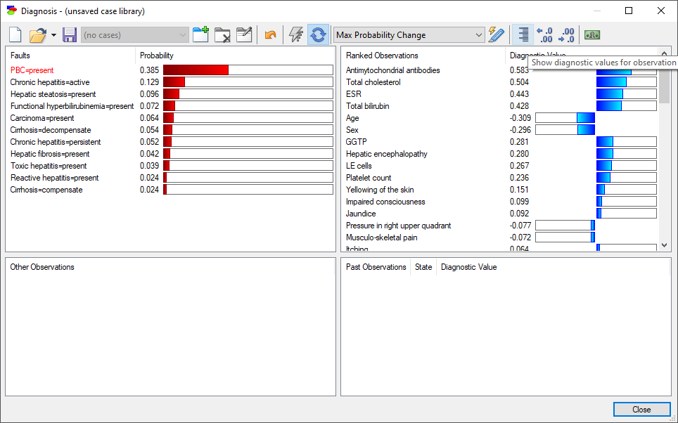
And so, there exists a state of the observation node Antimychondrial antibodies for which the probability of the state present of the node PBC (currently pursued fault) will increase by 0.583. Similarly, there exists a state of the node Age for which the probability of the currently pursued fault will decrease by 0.309. The maximum change is taken over the absolute values of the change in probability. Pressing the Show diagnostic values for observation outcomes button (![]() ) displays the probability change for each of the individual states of the observation nodes.
) displays the probability change for each of the individual states of the observation nodes.
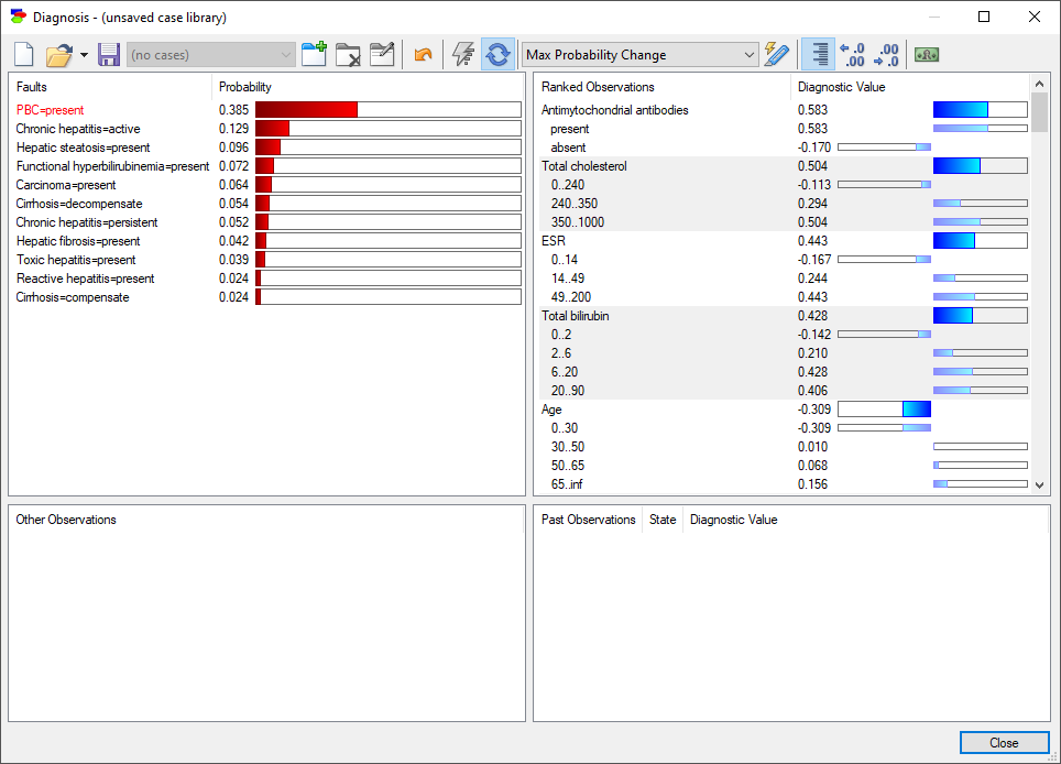
The expanded list allows to see which state exactly is capable of making the largest change in the probability of the pursued fault. And so, we can now see that the state present of the node Antimychondrial antibodies can increase the probability of the currently pursued fault by 0.583, while state absent can decrease it by 0.17. Similarly, state 0..30 of node Age will decrease the probability of the pursued fault by 0.309, while other states will generally increase the probability.
Cross-entropy
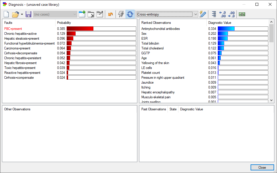
The insight from the Max Probability Change is limited in the sense of not telling us a key piece of information how likely each of the changes happens. For example, a positive test result for cancer will make a huge change it the probability of cancer. However, the probability of seeing a positive test may be very small in a generally healthy person. So, effectively the expected amount of diagnostic information from performing this test is rather small. Cross-entropy is an information-theoretic measure that takes into account both the amount of information flowing from observing individual states of an observation variable and the probabilities of observing this states. A high cross-entropy indicates a high expected contribution of observing a variable to the probability of the pursued fault. Here is the diagnostic window with cross-entropy of the individual observations:
Pressing the Show diagnostic values for observation outcomes button (![]() ) displays the entropy change for each of the individual states of the observation nodes.
) displays the entropy change for each of the individual states of the observation nodes.
We can see that cross-entropy, the expected change in entropy, is always in-between the changes in entropy due the individual states.
Normalized Cross-entropy
Normalized cross-entropy is essentially entropy divided by the current value of the entropy of the focus node. It is very similar to cross-entropy.
Measures of Diagnostic Value of Information for Multiple Pursued Faults
The meaning of each of the three measures is quite clear in case of pursuing a single fault or pursuing multiple faults that are various states of a single node. Additionally, the calculation of cross-entropy is exact in this case. When the pursued faults are located in various nodes, the calculation of exact cross-entropy is computationally hard, as it would require calculating the joint probability distribution over the pursued fault nodes. In this section, we will introduce the diagnostic measures of information used for multiple fault diagnosis. Multiple fault diagnosis is invoked by pursuing more than one fault.
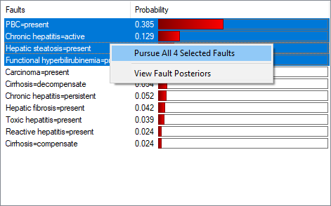
Once multiple faults are pursued, the selection of measures changes to a longer list
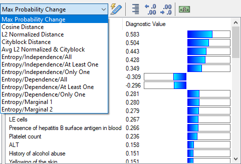
We will discuss each of these choices individually.
Max Probability Change
The extension of this measure to multiple faults amounts to taking the maximum change in the probability of a pursued fault over all pursued faults.
Cosine Distance
Cosine distance (also referred to as cosine similarity, https://en.wikipedia.org/wiki/Cosine_similarity) measures the distance between two vectors of numbers, in this case vectors of marginal probabilities of pursued faults, before and after making an observation. The larger the distance, the larger the impact of the observation. Cosine distance operates on vectors of probabilities and it naturally fits pursuit of multiple faults.
L2 Normalized Distance
L2 norm, also called Euclidean distance, Euclidean length, or L2 norm (https://en.wikipedia.org/wiki/Norm_(mathematics)#Euclidean_norm) calculates the distance between two vectors in Euclidean space. This measure also naturally fits pursuit of multiple faults.
Cityblock Distance
City block distance (https://en.wikipedia.org/wiki/City_block) calculates the distance between two points in multidimensional space. The points are expressed by two vectors of numbers, in this case vectors of marginal probabilities of pursued faults, before and after making an observation. The larger the distance, the larger the impact of the observation. City block distance is close to Euclidean distance but is better suited for discrete/rounded probabilities. It operates on vectors of probabilities and it naturally fits pursuit of multiple faults.
Avg L2 Normalized & Cityblock
This measure of distance takes the average between the L2 Normalized Distance and Cityblock Distance.
Entropy-based Measures
Because entropy-based measures require calculation of the joint probability distribution over all pursued faults, which is computationally prohibitive, it is necessary to use approximations of the joint probability distribution. The approximations are based on two strong assumptions about dependencies among them: (1) complete independence (this is taken by the first group of approaches) and (2) complete dependence (this is taken by the second group of approaches). Each of the two extremes is divided into three groups: (1) At Least One, (2) Only One, and (3) All. These refer to different partitioning of the combinations of diseases in cross-entropy calculation.
In practice, each of the approximations will give a reasonable order of tests but in cases where it is important to be precise about the order of tests, it may be a good idea to try all three because all three are approximations and it is impossible to judge which of the approximations is the best without knowing the joint probability distribution over the faults.
Entropy/Independence/All
The assumption is that the pursued faults are independent of each other, All means opposing the event that all faults are present against the event that at least one fault is absent.
Entropy/Independence/At Least One
The assumption is that the pursued faults are independent of each other, At Least One means opposing the event that at least one of the faults is present against the event that none of the faults are present.
Entropy/Independence/Only One
The assumption is that the pursued faults are independent of each other, Only One means opposing the event that exactly one fault is present against all other possibilities (i.e., multiple faults or no faults present).
Entropy/Dependence/All
The assumption is that the pursued faults are perfectly dependent on each other, All means opposing the event that all faults are present against the event that at least one fault is absent.
Entropy/Dependence/At Least One
The assumption is that the pursued faults are perfectly dependent on each other, At Least One means opposing the event that at least one of the faults is present against the event that none of the faults are present.
Entropy/Dependence/Only One
The assumption is that the pursued faults are perfectly dependent on each other, Only One means opposing the event that exactly one fault is present against all other possibilities (i.e., multiple faults or no faults present).
Entropy/Marginal 1/2
The Marginal probability-based approach is much faster than the independence/dependence-based joint probability distribution approaches but it is not as accurate because it makes a stronger assumption about the joint probability distribution. Entropy calculations in this approach are based purely on the marginal probabilities of the pursued faults. The two algorithms that use the Marginal Probability Approach differ essentially in the function that they use to select the tests to perform. Both functions are scaled so that they return values between 0 and 1.
Entropy/Marginal 1 uses a function without the support for maximum distance and its minimum is reached when all probabilities of the faults are equal to 0.5.
Entropy/Marginal 2 uses a function that has support for maximum distance and is continuous in the domain [0,1].
We would like to stress that none of the measures of distance supported by GeNIe (or any other systems for that matter) will offer optimality guarantees, i.e., guarantees that the order of tests suggested in the diagnosis dialog is optimal. Each of the measures will produce similar but not identical results and their optimality will depend on the model in which they are used (practically, depending on how well the model fits the assumptions made by each method). Users performing diagnosis interactively are encouraged to try several measures and pursue those observations that are indicated as the most informative consistently by various measures. When the models are embedded in end-user systems, we advise to select the measure that performs best in a given model. We recommend entropy-based methods in both single-fault and multiple fault diagnosis.
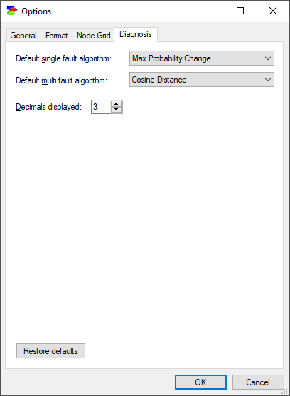
Please note that once you have become comfortable with different measures and develop preference for some of them, you can set the preferred measures of diagnostic values in the Diagnosis tab of program Options: