We will use the following simple model that demonstrates the geo-processing capability of GeNIe:
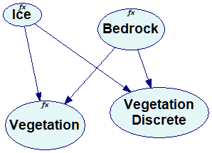
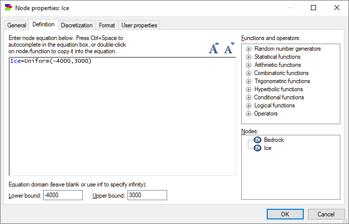
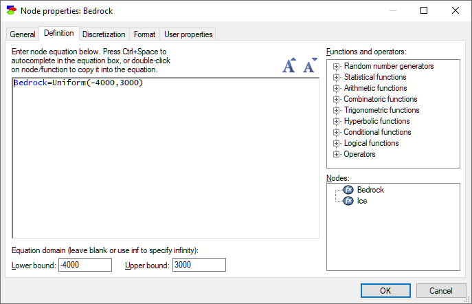
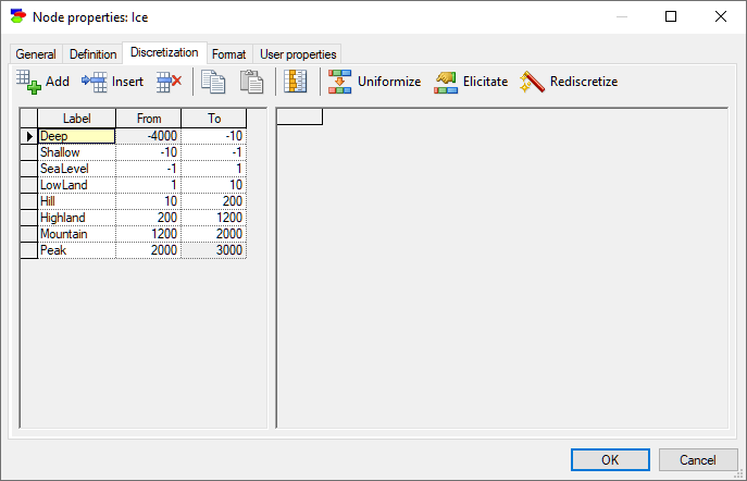
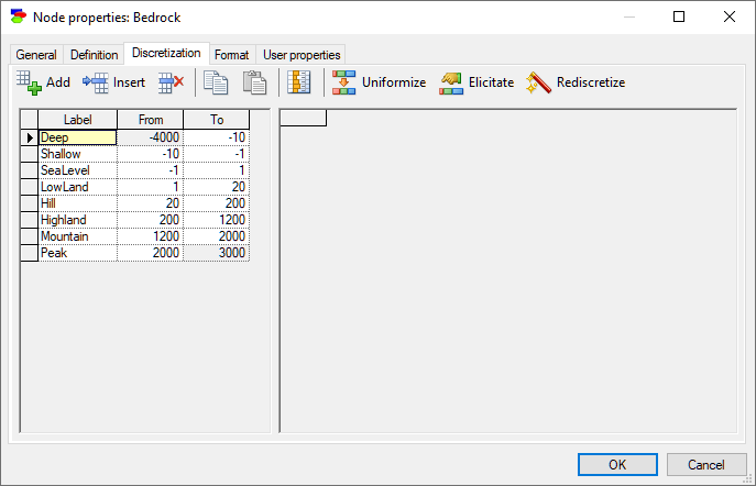
The model contains two variables that will take their values from maps (Ice and Bedrock) and two variables that will serve as values for the output maps (Vegetation and Vegetation Discrete). All variables, except for Vegetation Discrete are continuous. The definitions of the variables Ice and Bedrock are
The definition of the variable Vegetation is as follows
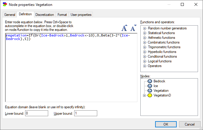
Essentially, perhaps somewhat naively, we have defined the probability of vegetation as a Beta distribution with the first parameter dependent on the difference between the level of ice and the bedrock, which amounts to the thickness of ice in that location. In all those areas that are more than 10 meters below the sea level and those areas in which the thickness of the ice cover is larger than 1 meter, the probability of vegetation is defined as zero.
The definition of the variable Vegetation Discrete is a conditional probability table derived from the definition of the variable Vegetation. For this purpose, we have discretized the variables Ice and Bedrock as follows
The resulting CPT of the variable Vegetation Discrete is as follows
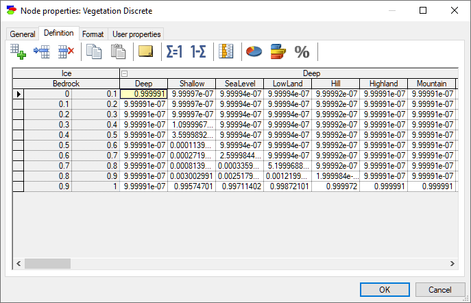
The two variables Vegetation and Vegetation Discrete are almost identical, with the variable Vegetation Discrete being a discrete version of the variable Vegetation.
Once we have opened all input map files and a model file (the model describes the interaction between the data in the input maps and the data in the output maps), we can invoke the dialog that allows us to describe the map processing. To that effect, we select Process... from the Geo Menu (or from the map context menu):
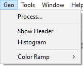
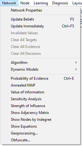
Another way of invoking the geo-processing is through the Geoprocessing... in the Network Menu.
This invokes the geo-processing dialog, which essentially allows us to tie the input maps with a Bayesian network model and specify the output maps.
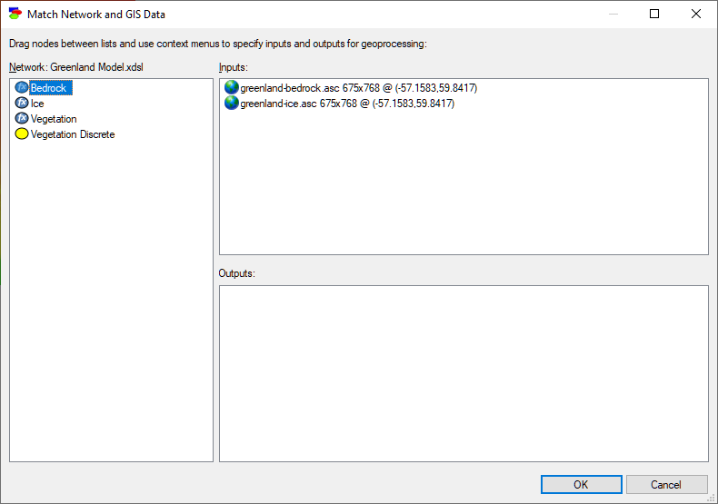
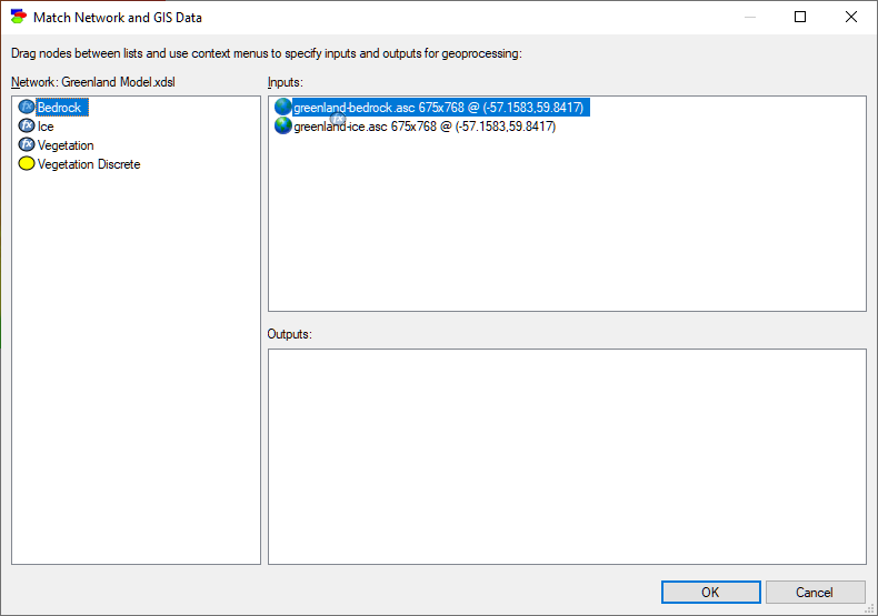
The dialog shows all maps that have been loaded into GeNIe (in this case, greenland-ice.asc and greenland-bedrock.asc) and all variables in the model chosen for geo-processing (in this case, Bedrock, Ice, Vegetation and Vegetation Discrete). To associate variables with input maps, we drag the variable name from the left-hand side pane to the upper-right-hand side pane and drop it in the corresponding map name. We drag and drop the variable Bedrock into the map greenland-bedrock.asc
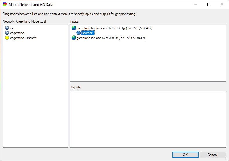
After the drop, the dialog shows an association between the variable and the map
While the meaning of this association is that the same raster cell in each of the maps is tied to the model variable, GeNIe allows also for associating model variables with neighboring map elements. This has application in all those situations in which the neighborhood of the current cell matters, for example in recognizing patterns in the maps. This way, the same map can have more than one variable associated with it, each variable associated to a different raster cell. The default association is the current cell. This can be changed by right-clicking on a variable associated with a map. For example, to change the offset of the variable Bedrock, please right-click on it and choose the offset (relative to the position of the current cell).
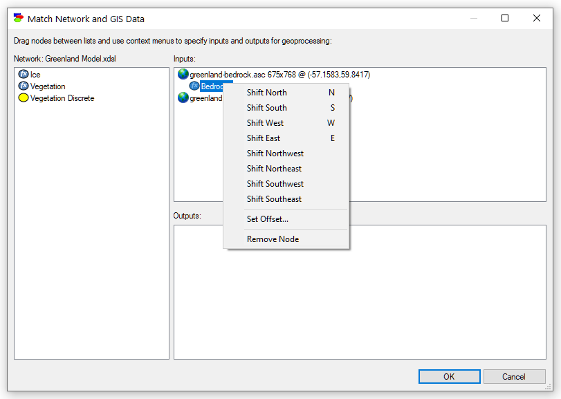
Set Offset... is the most general choice that allows for entering any offset in the x and y directions:
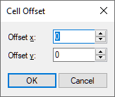
Offset (0,0) corresponds to the current cell, offset (0,1) corresponds to the cell above it, (-1,-1) to the cell to the left and below it, etc. Choices Shift North, Shift South, etc., are shortcuts that refer to the cells in the immediate neighborhood of the current cell. North, South, West, etc., describe a relative position with respect to the current cell. For example, North (N) is the cell above it (0,1), West (W) is the cell to the left of it (-1,0), Northeast is the cell up and to the right of the current cell. Since our simple example does not include any variables that are outside of the current cell, we leave the offset at (0,0).
We continue by associating the variable Ice with the map greenland-ice.asc (through dragging and dropping, as was the case for variable Bedrock) and dropping the variables Vegetation and Vegetation Discrete into the (lower right) Outputs pane. The resulting dialog looks as follows
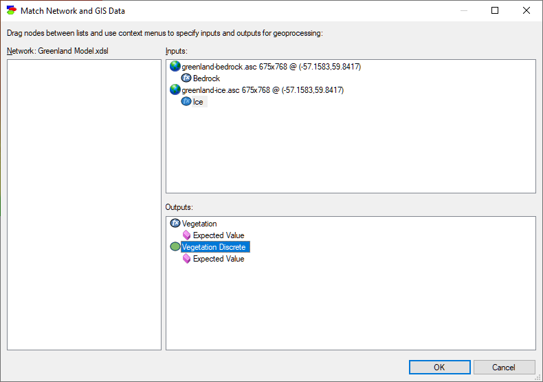
The dialog tells us that when processing the maps, greenland-bedrock.asc will provide input for the variable Bedrock, greenland-ice.asc will provide input to variable Ice, and there will be two output maps, Vegetation and Vegetation Discrete. One final step is deciding what values precisely should make it to the outputs maps. When the output variable is numerical (whether it is continuous or discrete), the default output is the expected value of the variable. In case of continuous variables, this is the only choice, as shown by right-clicking on the on the Expected Value text.
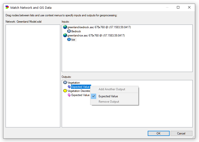
In case of discrete variables (whether numerical or categorical), there are additional choices:
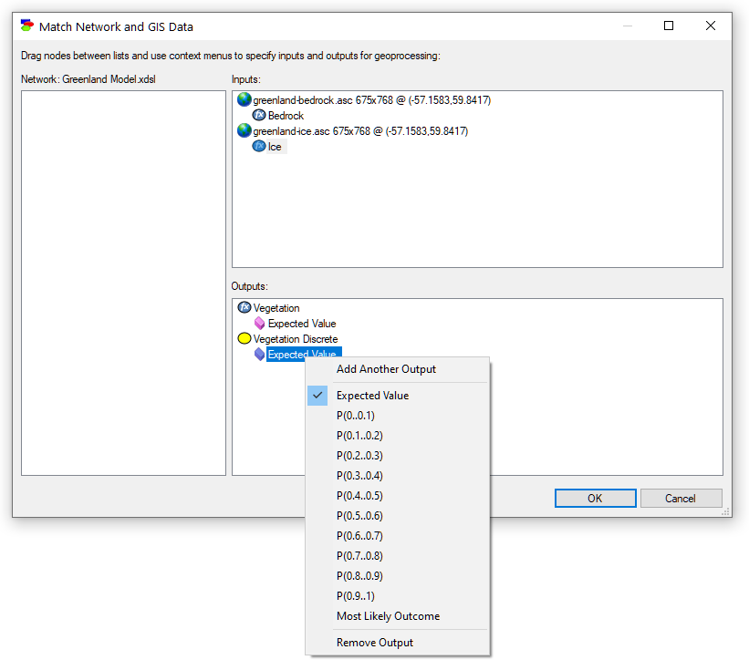
In addition to expected value (numerical variables only), we can select the probability of any of the discrete states or the most likely outcome.
We will leave the output type at the Expected Value for both maps. Clicking OK starts the processing
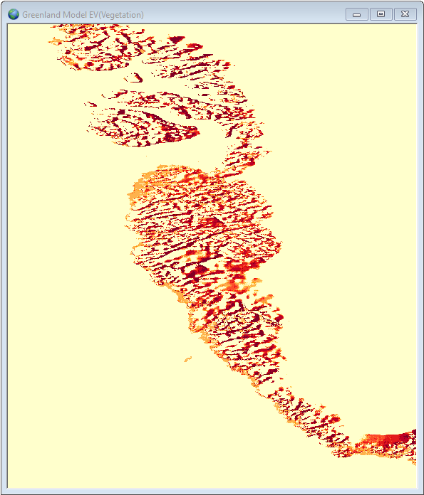
which end with two additional maps shown in GeNIe: Greenland Model EV(Vegetation)
and Greenland Model EV(VegetationD)
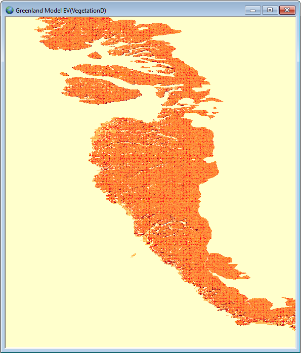
The two maps are similar, although one can see the impact of discretization on the Greenland Model EV(VegetationD) map. Both maps show for each raster cell the probability of vegetation, as defined in the Bayesian network model. We can see that generally only coastal areas of the map have non-zero probability of vegetation. The maps can be analyzed and/or saved for further processing.