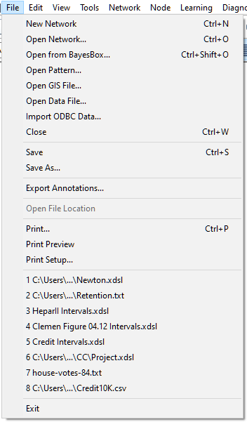
Equation-based models consist of Equation nodes. To construct an equation-based model, add Equation nodes to the Graph View and add connections between them. Let us create a simple model describing an object of mass m under influence of a force f, receiving acceleration a, which is governed by Newton's 2nd law of motion. We start by selecting New Network from the File Menu
We proceed by dropping three Equation nodes in the Graph View window using the Tools Menu
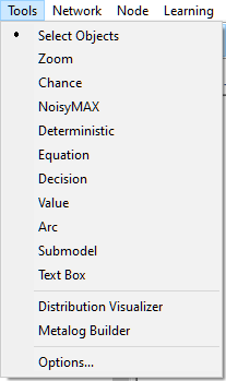
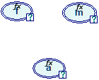
or the Equation (![]() ) button from the Standard Toolbar. We name them f, m, and a.
) button from the Standard Toolbar. We name them f, m, and a.
We define them as follows. Let the force be a constant (f=1) with some noise that we express by means of a Triangular(-0.1,0,0.1) distribution.
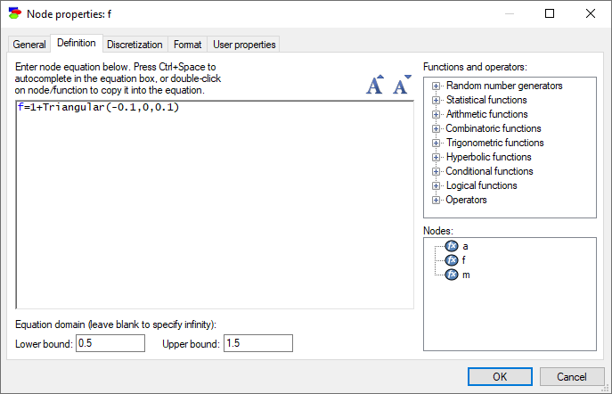
We specify the plausible domain of values of f to be between 0.5 and 1.5 Newtons.
Let the mass be a constant (m=5) with some noise that we express by means of a Uniform(-0.5,0.5) distribution.

We specify the plausible domain of values of m to be between 3 and 7 kilograms.
You may also select the definition of the node from a Quick definitions list at the time of creating a new equation node in the Graph View. To do so, select ![]() (Equation button) from the Standard Toolbar or Tools Menu. The Equation button will become recessed and the cursor will change to an arrow with an ellipse (with a wave sign) in bottom right corner. Move the mouse to a clear portion of the screen inside GeNIe window, hold the SHIFT key on the keyboard and click the left mouse button. The following menu with Quick definitions list for the nodes will pop up:
(Equation button) from the Standard Toolbar or Tools Menu. The Equation button will become recessed and the cursor will change to an arrow with an ellipse (with a wave sign) in bottom right corner. Move the mouse to a clear portion of the screen inside GeNIe window, hold the SHIFT key on the keyboard and click the left mouse button. The following menu with Quick definitions list for the nodes will pop up:
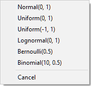
Selecting any of the items on the list creates nodes with the selected definition, which can be subsequently modified.
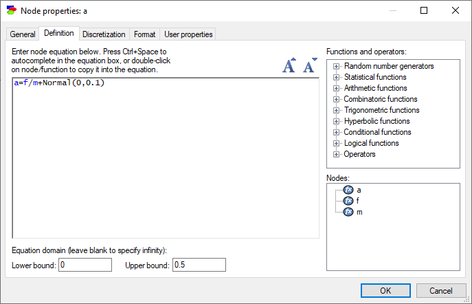
We define the third variable, acceleration a, as a function of f and m using Newton's 2nd law of motion and adding some noise, expressed by means of a Normal(0,0.1) distribution. We estimate the plausible domain of values of a to be between 0 and 0.5.
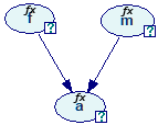
The graph of the model in the Graph View changes - arcs are added from the variables f and m to a.
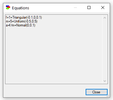
The model constructed corresponds to the following system of six simultaneous structural equations with six variables:
ε_f=Triangular(-0.1,0,0.1)
ε_m=Uniform(-0.5,0.5)
ε_a=Normal(0,0.1)
f=1+ε_f
m=5+ε_m
a=f/m+ε_a
The system could be simplified to three structural equations with three variables if we replaced variables ε with just references to probability distributions, like we did in the Bayesian network model constructed in this section. The distributions used (Triangular, Uniform, and Normal) may not be physically plausible in this example. We just wanted to use them to show that GeNIe puts no limitations on the functional form and the distributions used in the equations. Any function and any distribution available in the Functions and operators pane on the right-hand side can be used in the definition.
One can display the equations embedded into a hybrid model by choosing Show Equations from the Network Menu. This will display a dialog with all equations (in their simplified form) extracted from the model. The dialog invoked for the above model will look as follows: