Most systems in the world change over time and sometimes we are interested in how these systems evolve over time more than we are interested in their equilibrium states, as modeled by Bayesian networks. Whenever the focus of our reasoning is change of a system over time, we need a tool that is capable of modeling dynamic systems.
A dynamic Bayesian network (DBN) is a Bayesian network extended with additional mechanisms that are capable of modeling influences over time (Murphy, 2002). The temporal extension of BNs does not mean that the network structure or parameters changes dynamically, but that a dynamic system is modeled. In other words, the underlying process, modeled by a DBN, is stationary. A DBN is a model of a stochastic process. While Bayesian networks could be thought of as close relatives of systems of simultaneous equations, DBNs can be thought as close relatives of difference equations (difference rather than differential equations because time, as modeled in DBNs, is discrete).
The following example of a DBN originates from the doctoral research conducted by Dr. Anna Lupinska-Dubicka (2014) and is available from BayesFusion's interactive on-line model repository. It models woman's monthly cycle and helps with predicting the day of ovulation, with applications to fertility awareness and difficulties with conception.
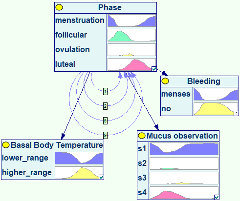
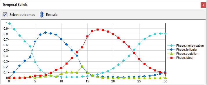
This DBN model allows for deriving probability distributions over variables of interest over time. The following plot shows the probabilities of various phases of the monthly cycle as a function of time given the observation of bleeding at time zero.
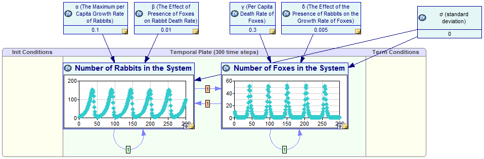
DBNs can include continuous nodes that are described by means of difference equations. In this case, the results derived by means of a DBN will resemble those obtained by solving the equations. Consider the well known predator-prey model introduced and studied theoretically by Alfred J. Lotka and later by Vito Volterra (see https://en.wikipedia.org/wiki/Lotka%E2%80%93Volterra_equations for more information). The model is based on two differential equations that describe how the population of prey and the population of predators depend on each other. A DBN model based on the Lotka-Volterra difference equations is capable of deriving the number of predators and prey as a function of time, as shown in the following screen shot of the model:
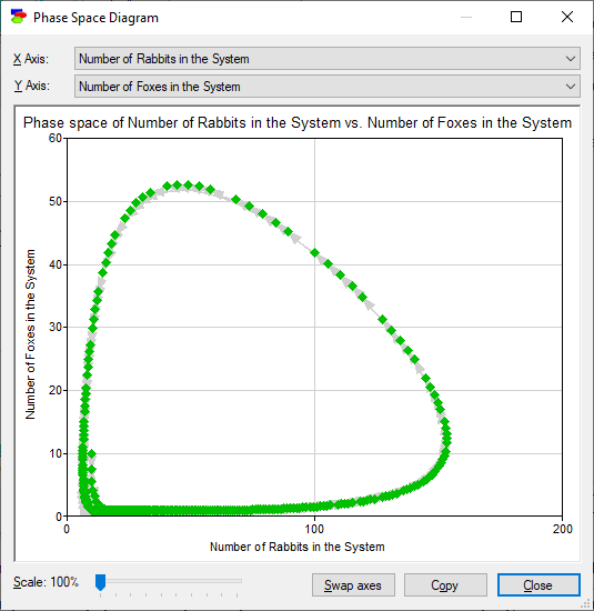
The model allows for deriving so-called phase-space diagrams, which are plots of the value of one variable as a function of another, in this case the number of foxes in a natural system as a function of the number of rabbits in the system:
The greatest advantage of a Dynamic Bayesian network model over a system of differential/difference equations is that solving the former is based on stochastic simulations rather than an analytical solution. This allows for modeling that is not constrained by what is solvable but rather focusing on the subject matter and the theoretical and practical aspects of the problem at hand. In addition to that, DBNs allow for injecting uncertainty into models and processing this uncertainty correctly. It also allows for entering observations at different time steps. The above plots are based on observing that there are 10 rabbits and 10 foxes at time zero.