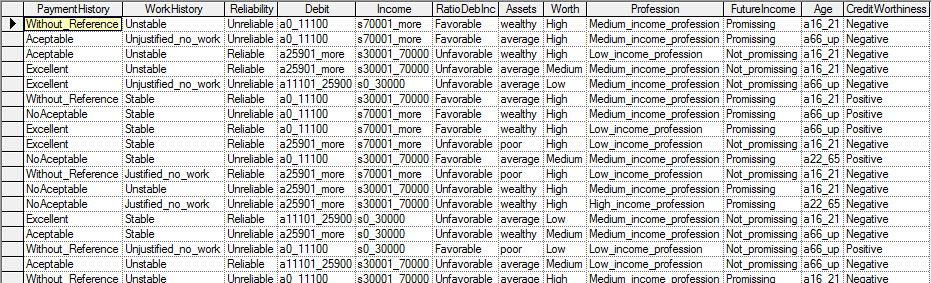
Suppose we have a file Credit10K.csv consisting of 10,000 records of customers collected at a bank. Each of these customers was measured on several variables, Payment History, Work History, Reliability, Debit, Income, Ratio of Debts to Income, Assets, Worth, Profession, Future Income, Age and Credit Worthiness. The file is too large to include in this manual, but it can be downloaded from https://support.bayesfusion.com/docs/Examples/Learning/Credit10K.csv. It is also included in the Examples\Learning directory of GeNIe installation. The first few records of the file (included among the example files with GeNIe distribution) look as follows in GeNIe:
We want to learn the structure of the Bayesian network based on the data. Our program attempts to load the data file from disk, and prints the number of data set variables and records if loading was successful.
DSL_dataset ds;
int res = ds.ReadFile("Credit10k.csv");
if (DSL_OKAY != res)
{
printf("Dataset load failed\n");
return res;
}
printf("Dataset has %d variables (columns) and %d records (rows)\n",
The most general structure learning algorithm is Bayesian Search. It is a hill climbing procedure with random restarts, guided by log-likelihood scoring heuristic. Its search space is hyper-exponential, so for best results the algorithm can be fine-tuned with multiple options (details are available in the Reference section). We set the number of iterations (random restarts) to 50, and fix the random number seed to ensure reproducible results. The DSL_bs::Learn method requires at least two parameters: (1) an input data set, and (2) an output network. We also want to record the log-likelihood of best structure among the 50 best structures created internally. The best structure will be copied into the output network, and parameter learning will be run internally. The output network will therefore be ready to use.
double bestScore;
DSL_bs bayesSearch;
bayesSearch.nrIteration = 50;
DSL_network net1;
bayesSearch.seed = 9876543;
res = bayesSearch.Learn(ds, net1, NULL, NULL, &bestScore);
if (DSL_OKAY != res)
{
printf("Bayesian Search failed (%d)\n", res);
return res;
}
net1.SimpleGraphLayout();
printf("1st Bayesian Search finished, structure score: %g\n", bestScore);
net1.WriteFile("tutorial9-bs1.xdsl");
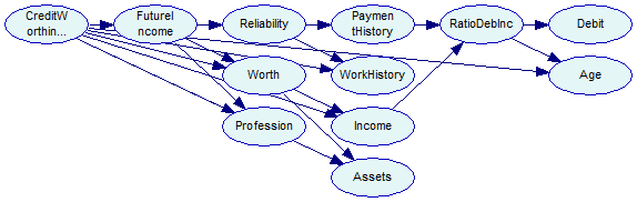
On success, we call DSL_network::SimpleGraphLayout to perform the parent ordering layout. Without this step, all nodes would occupy the same position and the structure would be hard to read when opened in GeNIe. The network looks as follows in GeNIe:
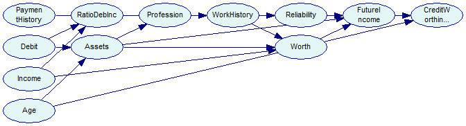
The network is saved for reference in the tutorial9-bs1.xdsl file. We can obtain a different structure by changing the seed for the random number generator and calling DSL_bs::Learn again.
DSL_network net2;
bayesSearch.seed = 3456789;
res = bayesSearch.Learn(ds, net2, NULL, NULL, &bestScore);
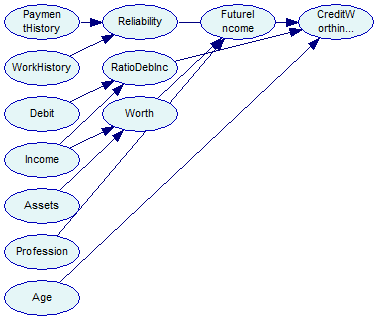
The second network, saved in tutorial9-bs2.xdsl, looks like this:
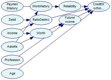
The log-likelihood scores for these two networks are -105473 and -105353, respectively.
Our third attempt at structure learning with Bayesian Search will use background knowledge. We want to forbid the arc between Age and CreditWorthiness, and force an arc between Age and Profession. When specifying the background knowledge, we refer to the data set variables as their indices, so we need to convert the textual identifiers to indices first with DSL_dataset::FindVariable:
int idxAge = ds.FindVariable("Age");
int idxProfession = ds.FindVariable("Profession");
int idxCreditWorthiness = ds.FindVariable("CreditWorthiness");
The forbidden and forced arcs now can be specified before DSL_bs::Learn call.
bayesSearch.bkk.forbiddenArcs.push_back(make_pair(idxAge, idxCreditWorthiness));
bayesSearch.bkk.forcedArcs.push_back(make_pair(idxAge, idxProfession));
res = bayesSearch.Learn(ds, net3, NULL, NULL, &bestScore);
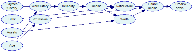
The output network now looks as follows - please note the absence of an arc from Age to CreditWorthiness, and the forced arc between Age and Profession.
We now change our learning algorithm to Tree Augmented Naive Bayes (TAN), implemented in SMILE in DSL_tan class. The TAN algorithm starts with a Naive Bayes structure (i.e., one in which the class variable is the only parent of all remaining, feature variables) and adds connections between the feature variables to account for possible dependence between them, conditional on the class variable. The algorithm imposes the limit of only one additional parent of every feature variable (additional to the class variable, which is a parent of every feature variable). We need to specify the class variable with its textual identifier. In this example CreditWorthiness is the class variable.
DSL_network net4;
DSL_tan tan;
tan.seed = 777999;
tan.classvar = "CreditWorthiness";
res = tan.Learn(ds, net4);
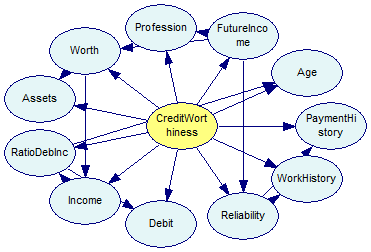
The program saves the network for reference in tutorial9-tan.xdsl file. The network looks as follows:
The layout of the TAN output network in our tutorial program does not take the specifics of the TAN into account. The same network looks like this when more sophisticated layout algorithm in GeNIe is used. The distinction between class and feature variables is now clearer.
Our final structure learning algorithm will be PC, which uses independences observed in data (established by means of classical independence tests) to infer the structure that has generated them. SMILE class implementing the PC algorithm is DSL_pc. The output of the PC algorithm is a pattern (represented by the DSL_pattern class). The pattern is an adjacency matrix, which does not necessarily represent a directed acyclic graph (DAG). The pattern can be converted to DSL_network with DSL_pattern::ToNetwork, which enforces the DAG criterion on the pattern, and copies the variables and edges to the network.
DSL_pc pc;
DSL_pattern pattern;
res = pc.Learn(ds, pattern);
if (DSL_OKAY != res)
{
printf("PC failed (%d)\n", res);
return res;
}
DSL_network net5;
pattern.ToNetwork(ds, net5);
At this point our output network has nodes with outcomes based on the labels in the data set, but the probability distributions in node definitions are uniform over outcomes. To complete the learning process, we need to manually call a parameter learning procedure implemented in DSL_em class.
DSL_em em;
string errMsg;
vector<DSL_datasetMatch> matching;
res = ds.MatchNetwork(net5, matching, errMsg);
if (DSL_OKAY != res)
{
printf("Can't automatically match network with dataset: %s\n", errMsg.c_str());
return DSL_OUT_OF_RANGE;
}
em.SetUniformizeParameters(false);
em.SetRandomizeParameters(false);
em.SetEquivalentSampleSize(0);
res = em.Learn(ds, net5, matching);
Note the DSL_dataset::MatchNetwork call, which populates the matching variable using identifiers of data set variables and network nodes. This information is subsequently used by DSL_em::Learn to associate data set variables with network node. The output network looks like as follows:
The network is saved for reference in the tutorial9-pc-em.xdsl file and Tutorial 9 finishes.