Consider the following example, inspired by (Russell & Norvig, 1995), in which a security guard at some secret underground installation works on a shift of seven days and wants to know whether it is raining on the day of her return to the outside world. Her only access to the outside world occurs each morning when she sees the director coming in, with or without an umbrella. Furthermore, she knows that the government has two secret underground installations: one in Pittsburgh and one in the Sahara, but she does not know which one she is guarding. For each day t, the set of evidence contains a single variable Umbrellat (observation of an umbrella carried by the director) and the set of unobservable variables contains Raint (a propositional variable with two states true and false, denoting whether it is raining) and Location (with two possible states: Pittsburgh and Sahara). The prior probability of rain depends on the geographical location and on whether it rained on the previous day. For simplicity, we do not use the initial and terminal condition nodes in this tutorial.
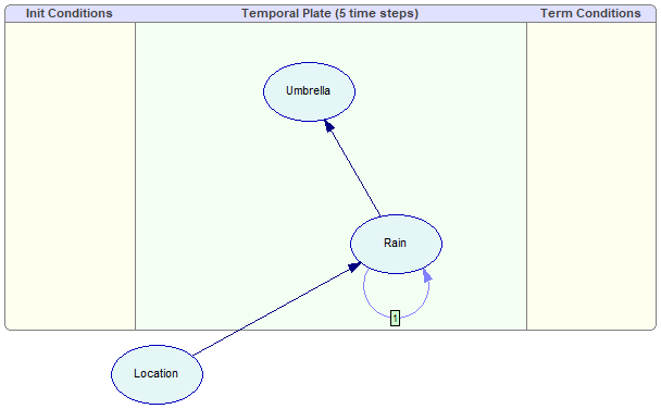
The model contains three discrete chance nodes (CPT), created with a call to CreateCptNode helper function, just like in nodes in Tutorial 1. The Rain and Umbrella nodes are marked as belonging to the temporal plate by calling DSL_network::SetTemporalType:
net.SetTemporalType(rain, dsl_temporalType::dsl_plateNode);
net.SetTemporalType(umb, dsl_temporalType::dsl_plateNode);
Two of the three arcs in the model are created by DSL_network::AddArc. We create the temporal arc expressing the dependency of Raint on Raint-1 by the AddTemporalArc method. Please note the temporal order of the arc passed as the 3rd parameter:
net.AddArc(loc, rain);
net.AddTemporalArc(rain, rain, 1);
net.AddArc(rain, umb);
CPTs for the nodes are initialized with DSL_nodeDef::SetDefinition, as in Tutorial 1. However, the node Rain requires two CPTs, because it has an incoming temporal arc of order 1. The first CPT is initialized with a call to DSL_nodeDef::SetDefinition, the second (temporal) CPT is initialized DSL_nodeDef::SetTemporalDefinition:
res = rainDef->SetTemporalDefinition(1, {
0.7, // P(Rain=true |Location=Pittsburgh,Rain[t-1]=true)
0.3, // P(Rain=false|Location=Pittsburgh,Rain[t-1]=true)
0.3, // P(Rain=true |Location=Pittsburgh,Rain[t-1]=false)
0.7, // P(Rain=false|Location=Pittsburgh,Rain[t-1]=false)
0.001, // P(Rain=true |Location=Sahara,Rain[t-1]=true)
0.999, // P(Rain=false|Location=Sahara,Rain[t-1]=true)
0.01, // P(Rain=true |Location=Sahara,Rain[t-1]=false)
0.99 // P(Rain=false|Location=Sahara,Rain[t-1]=false)
});
Finally, we adjust the number of slices created during the network unrolling with DSL_network::SetNumberOfSlices:
net.SetNumberOfSlices(5);
The network is complete. The program proceeds with a call to an inference algorithm, first without any evidence in the network, then with two observations of the Umbrella, set in the time steps t=1 and t=3:
net.GetNode(umb)->Val()->SetTemporalEvidence(1, 0);
net.GetNode(umb)->Val()->SetTemporalEvidence(3, 1);
Note that DSL_nodeVal::SetTemporalEvidence does not have the overload that takes an outcome identifier (a string) as 2nd argument. We need to provide an integer outcome index. In this case, we know that Umbrella outcomes are true at index 0 and false at index 1, because we created this node at the start of this tutorial.
In dynamic Bayesian networks, the plate nodes have their beliefs calculated for each time slice. The number of elements in the node value matrix for these nodes is the product of outcome count and slice count. The helper function UpdateAndShowTemporalResults iterates over this matrix using two nested loops in order to print the results:
const DSL_Dmatrix *mtx = node->Val()->GetMatrix();
for (int sliceIdx = 0; sliceIdx < sliceCount; sliceIdx++)
{
printf("\tt=%d:", sliceIdx);
for (int i = 0; i < outcomeCount; i++)
{
printf(" %f", (*mtx)[sliceIdx * outcomeCount + i]);
}
printf("\n");
}
Because the probabilities for the same slice are adjacent, the inner loop uses the product of the outcome count and slice index from the outer loop as a base index.
The dynamic network is saved to a file for future reference. If you want to explore the structure of the unrolled dynamic model, load the tutorial6.xdsl file into GeNIe and use the 'Unroll' command. Please compare the unrolled network with a more complex dynamic network described in the Unrolling section.
Tutorial 6 ends here.