Random number generators each generate a single sample from the distributions defined below. In most equations, they can be imagined as random noise that distorts the equation. Because the fundamental algorithm for inference in continuous and hybrid models is stochastic simulation, it is possible to visualize what probability distributions these single samples result in for each of the variables in the model.
Caution: Probability distributions are not allowed in expression-based MAU nodes, as these are deterministic functions by definition.
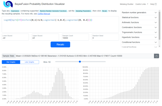
Choosing the right probability distribution over continuous data is a skill that requires some statistical insight. When the distribution is transformed by an equation expression, the task is daunting even for an experienced decision analyst. GeNIe offers an interactive tool for visualizing expressions, the Distribution Visualizer, with probability distributions through Monte Carlo simulation. The same functionality is available online at https://prob.bayesfusion.com. The screenshot below shows the online visualizer with the probability distribution sampled from the expression Log10(Sqrt(If(Uniform(0,1)<1/4,Lognormal(-1,0.3),Lognormal(0, 0.2)))).
Bernoulli(p)
Bernoulli is a discrete distribution that generates 0 with probability 1-p and 1 with probability p. Bernoulli(0.2) will generate a single sample (0 or 1) from the following distribution, i.e., 1 with probability 0.2 and 0 with probability 0.8:
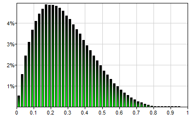
Beta(a,b)
The Beta distribution is a family of continuous probability distributions defined on the interval [0, 1] and parametrized by two positive shape parameters, a and b (typically denoted by α and β), that control the shape of the distribution. Beta(2,5) will generate a single sample from the following distribution:
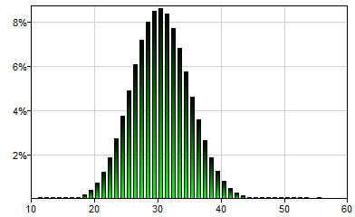
Binomial(n,p)
Binomial is a discrete probability distribution over the number of successes in a sequence of n independent trials, each of which yields a success with probability p. It will generate a single sample, which will be an integer number between 0 and n. A success/failure experiment is also called a Bernoulli trial. Hence, Binomial(1,p) is equivalent to Bernoulli(p). Binomial(100,0.3) will generate a single sample from the following distribution:
CustomPDF(x1,x2,...y1,y2,...)
The CustomPDF distribution allows for specifying a non-parametric continuous probability distribution by means of a series of points on its probability density (PDF) function. Pairs (xi,yi) are coordinates of such points. The total number of parameters of CustomPDF function should thus to be even. Please note that x coordinates should be listed in increasing order. The PDF function specified does not need to be normalized, i.e., the area under the curve does not need to add up to 1.0. For example, CustomPDF(0,1.02,1.9,3.2,10,0,4,5,1,0) generates a single sample from the following distribution:
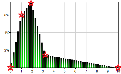
Stars on the plot mark the points defined by the CustomPDF arguments, i.e., (0, 0), (1.02, 4), (1.9, 5), (3.2, 1), and (10, 0).
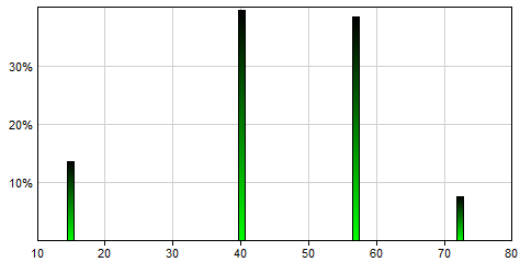
Discrete(x1,x2,...,xn, p1,p2,...,pn)
The Discrete distribution allows for specifying a discrete probability distribution over a collection of numerical values. It is one of the simplest random number generators, essentially replicating a discrete distribution and producing values x1, x2, ..., xn with probabilities p1, p2, ..., xn. This distribution is useful in simulating a discrete node using an equation node. The total number of parameters of Discrete() function should be even. Please note that x values should be listed in increasing order. Even though the p values should in theory add up to 1.0 and we advise that they do, GeNIe perform normalization, i.e., modifies them proportionally to add up to 1.0. For example, Discrete(15,40,57.5,72.5,0.137339,0.397711,0.387697,0.0772532) replicates the definition of the variable Age in the HeparII model and generates a single sample from the following distribution:
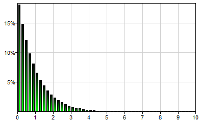
Exponential(lambda)
The exponential distribution is a continuous probability distribution that describes the time between events in a Poisson process, i.e., a process in which events occur continuously and independently at a constant average rate. Its only real-valued, positive parameter lambda (typically denoted by λ) determines the shape of the distribution. It is a special case of the Gamma distribution. Exponential(lambda) generates a single sample from the domain (0,∞). Exponential(1) will generate a single sample from the following distribution:
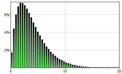
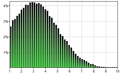
Gamma(shape,scale)
The Gamma distribution is a two-parameter family of continuous probability distributions. There are different parametrizations of the Gamma distribution in common use. SMILE parametrization follows one of the most popular parametrizations, with shape (often denoted by k) and scale (often denoted by θ) parameters, both positive real numbers. Gamma(2.0,2.0) will generate a single sample from the following distribution:
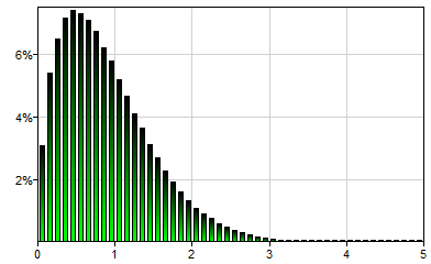
Lognormal(mu,sigma)
The lognormal distribution is a continuous probability distribution of a random variable, whose logarithm is normally distributed. Thus, if a random variable X is lognormally distributed, then a variable Y=Ln(X) has a normal distribution. Conversely, if Y has a normal distribution, then X=eY has a lognormal distribution. A random variable which is lognormally distributed takes only positive values. Lognormal(0,0.5) will generate a single sample from the following distribution:
Metalog(lower,upper,k,x1,x2,...,y1,y2,...)
Metalog (also known as the Keelin) distribution is a very flexible distribution, capable of fitting many naturally occurring distributions. It can be specified by probability quantiles, which are values of the variable xi and their corresponding cumulative probabilities yi. Metalogs are able to represent distributions that are unbounded, semi-bounded, and bounded. lower and upper are the bounds of the distribution (-Inf() and Inf() denote lower and upper infinite bound respectively). k is a parameter of the metalog distribution, running from 2 to n, where n is the number of probability quantiles specified. Generally the higher the value of k, the more flexible the distribution but it is worth looking at the distributions generated for different values of k to find a compromise between complexity and goodness of fit. The choice of k is best performed interactively, looking at the family of metalog distributions generated from the probability quantiles. GeNIe contains a built-in tool, the Metalog Builder, which displays metalog PDF and CDF charts. This functionality is also available online at https://metalog.bayesfusion.com.
The examples below use identical bounds and probability quantiles with k equal 4, 6 and 8:
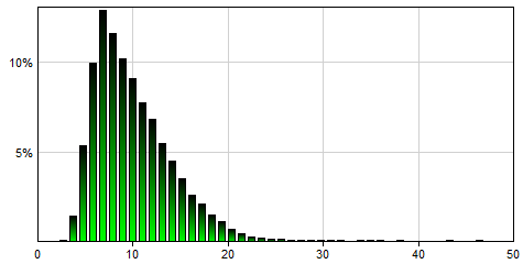
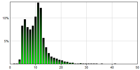
Metalog(0,Inf(),4,3,4,5,5,7,10,12,15,18,32,0.001,0.01,0.05,0.1,0.25,0.5,0.75,0.9,0.95,0.999) will generate a single sample from the following distribution:
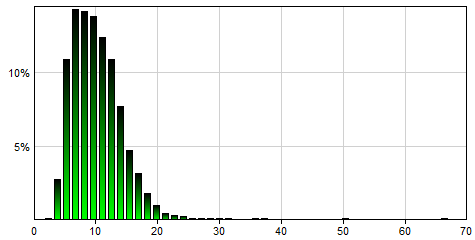
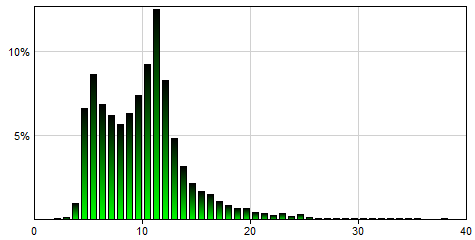
Metalog(0,Inf(),6,3,4,5,5,7,10,12,15,18,32,0.001,0.01,0.05,0.1,0.25,0.5,0.75,0.9,0.95,0.999) will generate a single sample from the following distribution:
Metalog(0,Inf(),8,3,4,5,5,7,10,12,15,18,32,0.001,0.01,0.05,0.1,0.25,0.5,0.75,0.9,0.95,0.999) will generate a single sample from the following distribution:
For more information about metalog distributions, please look at the comprehensive article on the topic on Wikipedia (https://en.wikipedia.org/wiki/Metalog_distribution), the Metalog Distribution web site created by Tom Keelin (http://metalogdistributions.com/) or the Metalog Distributions YouTube channel (https://www.youtube.com/channel/UCyHZ5neKhV1mSsedzDBoqyA).
MetalogA(lower,upper,a1,a2,...)
MetalogA function uses what one could call internal metalog coefficients (ai and, additionally, the lower and upper bound of the distribution) that, contrary to percentiles of the distribution used as parameters of Metalog, do not have easily interpretable meaning. One might expect that MetalogA is more efficient in sample generation, as it skips the whole process of deriving the distribution from which it subsequently generates a sample. However, SMILE has an efficient caching scheme that makes Metalog equally efficient in practice.
MetalogA(0,Inf(),2.30769,0.164148,-0.731388,0.343231,0.883249,-0.170727,1.40341,2.64853), which is equivalent to Metalog(0,Inf(),8,3,4,5,5,7,10,12,15,18,32,0.001,0.01,0.05,0.1,0.25,0.5,0.75,0.9,0.95,0.999), will generate a single sample from the following distribution:
Please note that the number of ai parameters of MetalogA is the same as the k parameter in Metalog. Obtaining the parameters ai outside of tools like Metalog Builder is rather challenging.
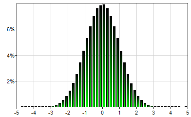
Normal(mu,sigma)
Normal (also known as Gaussian) distribution is the most commonly occurring continuous probability distribution. It is symmetric and defined over the real domain. Its two parameters, mu (mean, μ) and sigma (standard deviation, σ), control the position of its mode and its spread respectively. Normal(0,1) will generate a single sample from the following distribution:
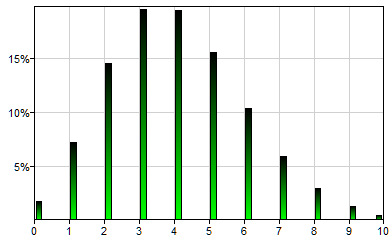
Poisson(lambda)
Poisson distribution is a discrete probability distribution typically used to express the probability of a given number of events occurring in a fixed interval of time or space if these events occur with a known constant rate and independently of the time since the last event. Its only parameter, lambda, is the expected number of occurrences (which does not need to be integer). Poisson(4) will generate a single sample from the following distribution:
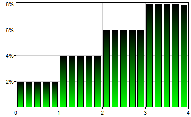
Steps(x1,x2,...y1,y2,...)
The Steps distribution allows for specifying a non-parametric continuous probability distribution by means of a series of steps on its probability density (PDF) function. It is similar to the CustomPDF function, although it does not specify the inflection points but rather intervals and the height of a step-wise probability distribution in each of the intervals. Because the number of interval borders is always one more than the number of intervals between them, the total number of parameters of Steps function should be odd. Please note that x coordinates should be listed in increasing order. The PDF function specified does not need to be normalized, i.e., the area under the curve does not need to add up to 1.0.
Example: Steps(0,1,2,3,4,1,2,3,4) generates a single sample from the following distribution::
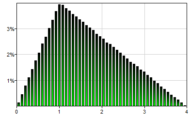
Triangular(min,mod,max)
Triangular distribution is a continuous probability distribution with lower limit min, upper limit max and mode mod, where min ≤ mod ≤ max. Triangular(0,1,3) will generate a single sample from the following distribution:
TruncNormal(mu,sigma,lower[,upper])
Truncated Normal distribution is essentially a Normal distribution that is truncated at the values lower and upper. This distribution is especially useful in situation when we want to limit physically impossible values in the model.
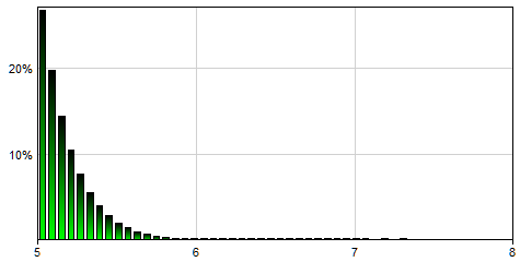
TruncNormal(3,2,1) will generate a single sample from the following distribution:
TruncNormal(0,1,5,10) will generate a single sample from the following distribution:
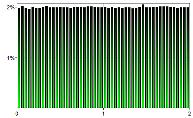
Uniform(a,b)
The continuous uniform distribution, also known as the rectangular distribution, is a family of probability distributions under which any two intervals of the same length are equally probable. It is defined two parameters, a and b, which are the minimum and the maximum values of the random variable. Uniform(0,2) will generate a single sample from the following distribution:
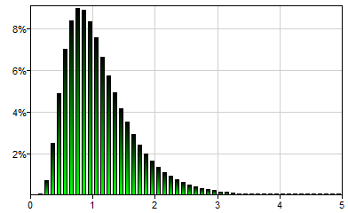
Weibull(lambda,k)
Weibull distribution is a continuous probability distribution named after a Swedish mathematician Waloddi Weibull, used in modeling such phenomena as particle size. It is characterized by two positive real parameters: the scale parameter lambda (λ) and the shape parameter k. Weibull(1,1.5) will generate a single sample from the following distribution: