Inference in a DBN, similarly to inference in a BN, amounts to calculating the impact of observation of some of its variables on the probability distribution over other variables. The additional complication is that both evidence and the posterior probability distribution is indexed by time. We will go through the example used in the previous sections to demonstrate setting evidence, running an algorithm, and viewing the results.
Setting temporal evidence
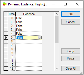
We can enter into the Product Temporal.qdsl model evidence stating that the initial six months of the time horizon the product s going to be of poor quality. This means that the evidence vector for the node High Quality of the Product is as follows:
High Quality of the Product[0:6]= [false, false, false, false, false, false].
To enter this evidence, we right-click on the High Quality of the Product node and select Evidence...
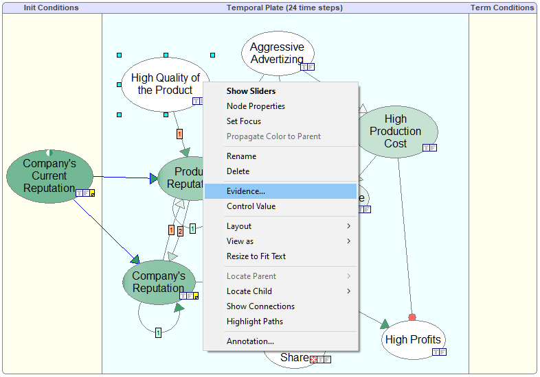
This invokes the Dynamic Evidence dialog
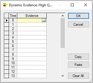
We enter the evidence vector as specified above:
Viewing results: Node gradients
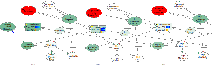
Once we exit the Dynamic Evidence dialog, QGeNIe calculates the impact of the observations. The following screen shot of the model shows how the truth of the propositions represented by the nodes changes with time.
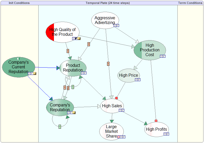
We can see that the first six months of poor quality product resulted in lower production costs but also in lowering the reputation of the product and lowering the company's reputation.
Viewing results: Active time step
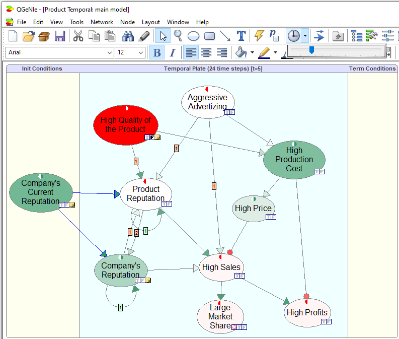
There is an additional, way of observing the results. QGeNIe allows for walking through the time steps and observing how the colors of nodes change. This is invoked by pressing the Active time step icon (![]() ). This shows a small slides for walking through the time steps.
). This shows a small slides for walking through the time steps.
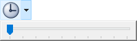
As we move the slider, the colors of nodes change. The following screen shot shows the colors (i.e., probabilities) at t=6. The time step is displayed in the header line of the temporal plate.
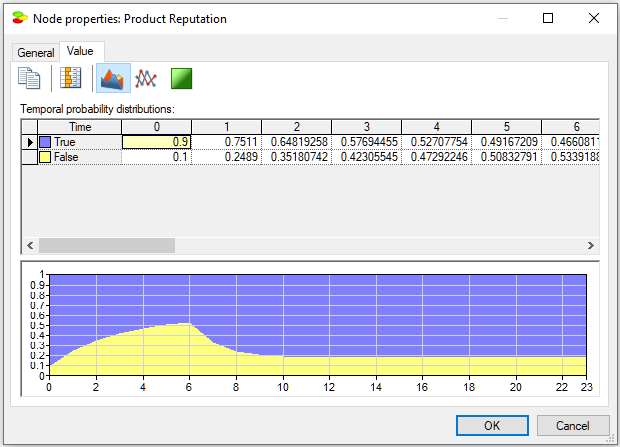
Viewing results: Value tab
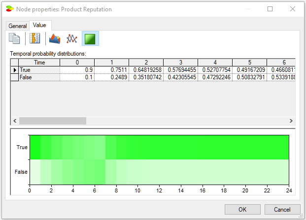
We can view the temporal beliefs in the Value Tab of a node as a spreadsheet indexed by the time steps. In addition to the numerical values of the marginal posterior probabilities over time, we can view the results graphically. Pressing the Area chart (![]() ) button displays the posterior marginal probabilities graphically:
) button displays the posterior marginal probabilities graphically:
Pressing the Contour plot (![]() ) button displays the posterior marginal beliefs as a contour plot with probabilities displayed by colors. Hovering over individual areas shows the numerical probabilities corresponding to the areas/colors.
) button displays the posterior marginal beliefs as a contour plot with probabilities displayed by colors. Hovering over individual areas shows the numerical probabilities corresponding to the areas/colors.
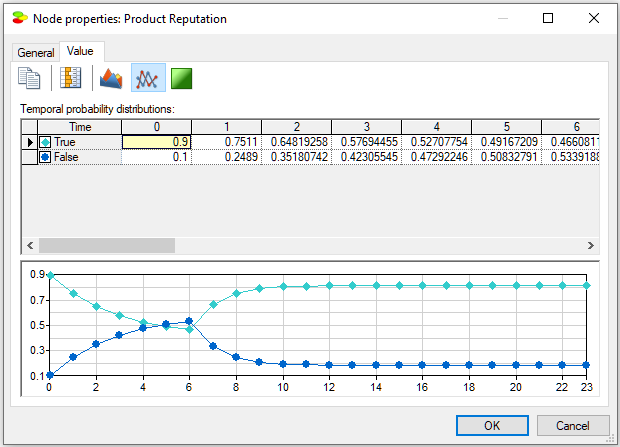
Finally, pressing the Time series (![]() ) button shows the posteriors as a time series plot (a curve for each of the two states of the variable):
) button shows the posteriors as a time series plot (a curve for each of the two states of the variable):
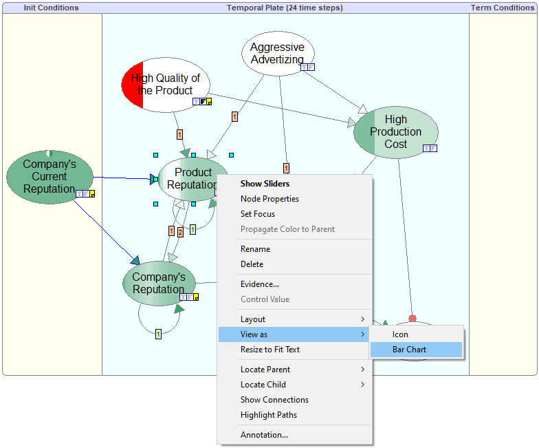
Viewing results: On-screen bar charts
Marginal posterior probabilities can be also shown on the screen permanently by the changing the node view to Bar chart. This can be accomplished by selecting nodes of interest and then changing the view of the nodes through the View as/Bar Chart option.
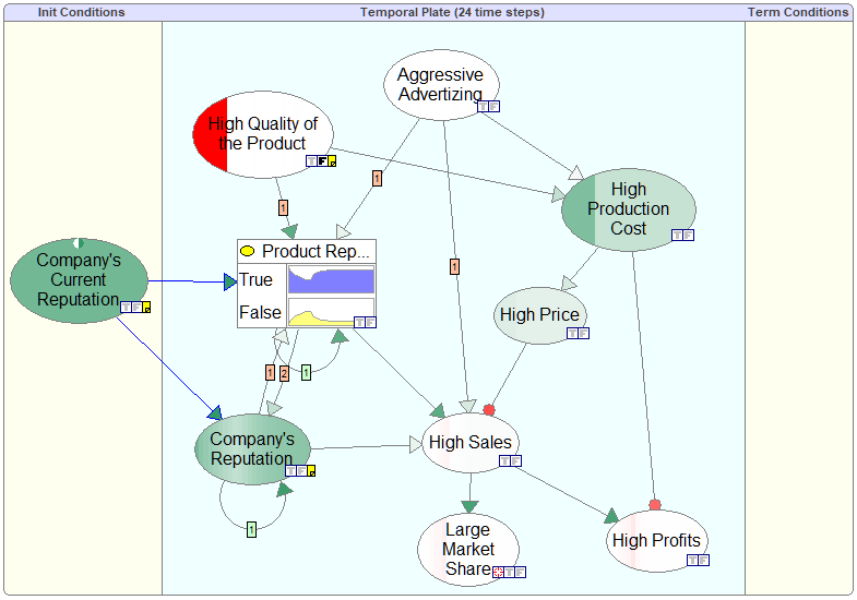
The Bar chart view allows for displaying the temporal posterior marginal probabilities on the screen permanently.
Viewing results: Temporal beliefs
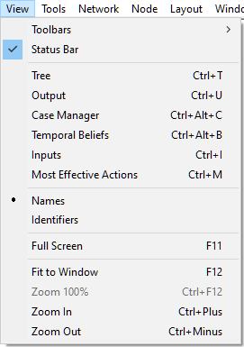
Marginal posterior probabilities can be also shown as a plot in a separate window called Temporal Beliefs. The Temporal Beliefs window can be opened by selecting it on the View menu.
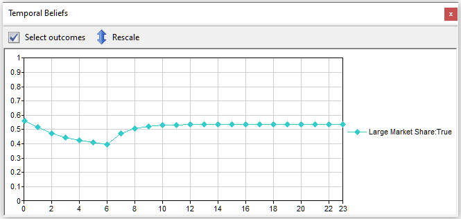
This opens the Temporal Beliefs window with the probability of the Focus node (in our model, it is the node Large Market Share) displayed
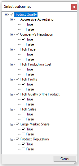
We can select propositions for which probabilities we want displayed by pressing the Select outcomes button on the top on this window. This pens a dialog that allows for selecting individual node states.
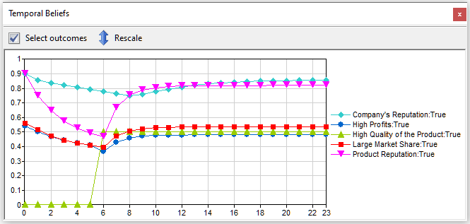
As we select states to be displayed, the Temporal Beliefs window shows them
Unrolling the DBN
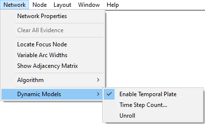
As we mentioned above, for the purpose of inference, QGeNIe converts the DBN into a Bayesian network and updates the beliefs using the selected belief updating algorithm. It can be useful, for example for model debugging purposes, to explicitly unroll a temporal network. QGeNIe provides this possibility through the Network-Dynamic Models-Unroll option.
QGeNIe creates a new network that has the temporal network unrolled for the specified number of time-slices. It is possible to locate a node in the temporal network from the unrolled network by right-clicking on the node in the unrolled network and selecting -> Locate Original in DBN from the context-menu. The unrolled network that is a result from unrolling the temporal network is cleared from any temporal information whatsoever. It can be edited, saved and restored just like any other static network. Figure below shows the unrolled network representation of a temporal network and how the original DBN can located back from the unrolled network.